Accurate dating of historical texts is essential for understanding cultural and historical narratives. However, traditional methods, such as paleographic and physical examination, can be subjective, costly, and potentially damaging to manuscripts. This paper introduces a machine learning approach to predicting the authorship dates of historical texts by using named entities — specifically, person and place names — as temporal markers. Using a dataset from Trismegistos, which includes metadata on the earliest and latest possible writing dates, we apply regression models to estimate text origins. While linear models like Lasso and Ridge Regression showed limited success, nonlinear models, including Random Forest, XGBoost, and Neural Networks, performed significantly better, with ensemble methods delivering the best results. The top-performing ensemble model achieved a mean absolute error of 45.7 years, surpassing traditional techniques. This study demonstrates the potential of named entities as temporal indicators and the effectiveness of ensemble learning in capturing complex historical patterns. Offering a scalable, non-destructive alternative to traditional methods.

1. Introduction

Accurate dating of historical texts and manuscripts remains a critical challenge for scholars, archivists, and curators, as it fundamentally shapes the understanding of historical narratives, cultural developments, and the evolution of ideas, yet traditional methods often fall short in providing precise chronological placement for many documents. This paper discusses the development and implementation of a machine learning based regression model designed to predict the year of origin for historical texts. Traditional historical manuscript dating (HMD) techniques, including paleographic and physical examination, present significant limitations due to their reliance on actual manuscript samples and their associated costs, time investment and potential for damage, motivating the exploration and development of modern computer-based alternatives [Omayio et al. 2022]. While direct physical techniques, such as radiocarbon dating [Jull et al. 1995], provide a means to compute the production date of historical manuscripts, they are destructive due to the use of a sample from the manuscript itself and can be affected by contaminants, leading to inaccuracies. In addition, methods such as radiocarbon dating provide the production date of writing support or material, which may not necessarily provide the authorship date of the content within the manuscript. Indirect physical techniques, such as spectroscopic methods, suffer from the same drawbacks. However, they offer the advantage of being non-destructive, but can still be influenced by modern pigments, leading to misleading conclusions regarding the manuscript’s age. The existence of such pigments can cast doubt on their authenticity and age, suggesting possible later modifications, restorations, or contamination [Castro et al. 2004] [Omayio et al. 2022]. Similarly, while paleographic analysis — which relies on the expertise of trained paleographers to assess handwriting styles and manuscript features — has historically been used for dating historical texts, this approach is often subjective, leading to inconsistencies and disagreements in dating conclusions among experts, therefore posing a challenge in the accuracy of historical manuscripts [Omayio et al. 2022]. Analyzing writing style is another method of dating ancient texts [Van Schaik 2013]. However, this method can also introduce inconsistencies and biases, limiting the reliability of findings. A machine learning approach to automatically analyze and date historic manuscripts can offer a more objective and efficient solution to this problem.

In this project, machine learning techniques were used to predict the year that a historical text was written, using named entities (person and place names) as key features. This approach is based on the premise that the presence of specific person and place names in a text can serve as temporal markers, helping to estimate the period in which the text was written.

A machine learning approach is particularly useful in the context of dating historical texts due to its ability to process large amounts of data efficiently, identify complex patterns, and provide objective, consistent results. Unlike traditional methods, machine learning can adapt to various languages and time periods and continuously improve as more data becomes available. This approach also offers a non-destructive alternative to physical dating methods, preserving valuable historical artifacts. By leveraging these advantages, machine learning techniques can significantly enhance the ability to date historical texts accurately and efficiently, contributing to a deeper understanding of historical narratives and cultural developments.

The dataset for this study consists of a one-hot encoded matrix of person and place names extracted from historical texts, alongside metadata specifying the earliest (y1) and latest (y2) possible writing dates. Since many records contain exact years (y1 = y2), a regression model to predict a specific year of authorship was best fit. However, for texts with uncertain dates (y1 ̸= y2), additional strategies were considered to refine the predictions. The objectives included exploring patterns in the data, handling date uncertainty, building a predictive model, and improving its accuracy through feature selection and ensemble techniques. To evaluate model performance, the mean absolute error was used. This study makes significant contributions to the fields of historical text dating and computational humanities. By leveraging named entity-based features, the research demonstrates their effectiveness as strong temporal indicators for predicting authorship dates. Furthermore, it highlights the power of ensemble learning in improving prediction accuracy. Additionally, the research provides valuable insights into the challenges associated with dating texts from specific time periods.

2. Related Work

Recent advancements in computational techniques have significantly enhanced the dating of historical texts and manuscripts. [Moscato et al. 2022] utilized a memetic algorithm-based Continued Fraction Regression (CFR) to date 181 Shakespeare-era plays (from 1585-1610), achieving a Mean Squared Error (MSE) of 21.25 by analyzing word frequency patterns, demonstrating the potential of regression-based methods for temporal prediction. Similarly, [Pavlopoulos et al. 2024] applied text regression to Greek papyri, achieving a mean absolute error of 54 years using extremely randomized trees, emphasizing textual features over subjective paleographical methods. [Hellwig 2019] employed supervised learning with linguistic features to date Classical Sanskrit texts, successfully classifying over 80% of the Bh¯ıs.maparvan’s adhy¯ayas, while [Yu and Huangfu 2019] leveraged bidirectional LSTM networks for ancient Chinese texts, achieving 95% accuracy without manual feature extraction.

Handwritten document recognition has also progressed, with [Ullah and Jamjoom 2022] achieving 96.78% accuracy in recognizing Arabic script using Convolutional Neural Networks (CNNs), addressing challenges posed by cursive forms and style variations. [Wahlberg et al. 2016] applied deep convolutional neural networks to premodern manuscripts, achieving a median absolute error of ±11.1 years, outperforming handcrafted feature methods (MSE 810-1389) with transfer learning and Sparse Gaussian Process regression. [He et al. 2014] introduced the Medieval Paleographic Scale (MPS) project, combining global and local regression for a mean absolute error of 35.4 years, while their 2016 study proposed a clustering algorithm (MLSOM) with a novel H2OS descriptor, yielding a mean absolute error of 15.9 years. [Hamid et al. 2018] fused textural features (Gabor, U-LBP, LBP) for a mean absolute error of 20.13 on the Medieval Paleographic Scale dataset, and [Koopmans et al. 2024] explored data augmentation with support vector machines, improving accuracy by 4.5% despite selective feature effectiveness.

[Kumar et al. 2011] applied a supervised language modeling approach to date fictional texts by capturing implicit temporal cues through Kullback-Leibler Divergence, achieving a median error of 23 years on Gutenberg short stories (1798–2008), thus refining document dating in narrative corpora. Similarly, [Han et al. 2023] introduced the Time-Aware Language Model (TALM), which incorporates temporal adaptation to align word representations across historical periods. Evaluated on Chinese and English corpora, TimeAware Language Model achieved an F1 score of 84.99% on the Twenty-Four Histories Corpus, surpassing state-of-the-art models in diachronic text analysis. Grapheme-based handwriting analysis using Self-Organizing Time Maps (SOTM) was employed by [Dhali et al. 2020] to cluster historical scripts, such as the Dead Sea Scrolls, into temporal categories, achieving a mean absolute error of 23.4 years. While outperforming traditional texture-based methods, the approach is constrained by its reliance on categorical classification and handwriting features, limiting its scalability across languages and document types.

[Assael et al. 2025] use a tool, Aeneas, a generative neural network for contextualizing ancient texts. Aeneas has a much broader scope than our project as its goals are to contextualize ancient texts and artifacts, going as far as performing restoration. As of the date published in the article, Aeneas currently focuses on Latin data.

3. Dataset

3.1. Origin of the dataset

The website Trismegistos, accessible at https://www.trismegistos.org, functions as a digital resource for investigating ancient civilizations across a broad geographic expanse, encompassing regions from Scandinavia to Ethiopia and from the Canary Islands to the Indus Valley, during the era from 800 BCE to 800 CE[Depauw 2018]. Originating from several research endeavors at KU Leuven, the platform initially concentrated on Egyptian papyri and other textual artifacts, with a particular focus on the individuals and locations they reference. The database has developed gradually, beginning with manual data input and periodic updates through partnerships with affiliated projects. More recently, it has integrated specially designed, rule-based Named Entity Recognition (NER) models to partially automate the extraction of references to people and places from comprehensive text repositories, such as those found on papyri.info [Broux and Depauw 2015] [Depauw and Van Beek 2009]. Each record in the dataset is meticulously structured and annotated, featuring extensive metadata that includes details on the text’s origin, chronological placement, language, genre, physical properties, and thematic content. This detailed metadata empowers scholars to examine and interpret the texts within their respective historical, linguistic, cultural, and geographic frameworks. Academics and specialists from a variety of disciplines — ranging from archaeology and history to philology, linguistics, and digital humanities — utilize the Trismegistos dataset for diverse research goals. The platform serves as a crucial instrument for exploring ancient societies, their economic frameworks, religious practices, languages, and cross-cultural dynamics, thereby offering a deeper comprehension of the multifaceted nature of life in the ancient world.

3.2. Structure of the dataset

The dataset obtained from Trismegistos comprises a comprehensive collection of features that describe historical texts. It was processed to a one-hot encoded manner, i.e., categorical data present in the dataset was represented by binary values, with “1” indicating the presence of a feature and “0” indicating its absence. The dataset includes a total of 11,599 unique person names and 4,784 place names, each formatted with a specific identifier. Each text entry is uniquely identified by a text ID, which serves as a reference point for the associated features.

In addition to the features, the dataset contains corresponding labels that provide information regarding the approximate date range of each text’s creation. Key variables within the labels represent this date range: one variable serves as the approximate start date (y1), while another serves as the approximate end date (y2). When y1 equals y2, it indicates the exact year of creation of the ancient text. The one-hot encoded dataset consists of 30,324 rows (texts) and 16,383 columns (features).

The labels (year of writing) included 29,250 rows, containing the dependent variables (y1 and y2) that the models aim to predict. These labels provide the reference values against which the model’s predictions are evaluated during both training and testing phases. This dataset is structured to facilitate effective training and evaluation of machine learning models for historical text dating.

Proper alignment between the datasets was a critical preprocessing step. Each text sample was associated with a unique identifier (text ID), which was used to match corresponding entries across both datasets. As some entries in the feature set did not have matching labels, and vice versa, an inner join was performed using this identifier to retain only the samples present in both datasets. Following this alignment, the resulting dataset comprised 8,565 entries, each containing both feature representations and their corresponding labels.

4. Methodology

4.1. Preprocessing and Data Exploration

For most models, additional scaling was unnecessary. However, for the neural network, StandardScaler was applied to transform each feature to have zero mean and unit variance. This step was important for mitigating issues such as vanishing or exploding gradients and ensuring compatibility with normal weight initialization. The target variable y was normalized to the range using MinMaxScaler, aligning with the linear output activation function and mean absolute error loss function employed during training.

Since the features were highly sparse, low-variance features were filtered using a threshold of 0.001. This process significantly reduced the feature space from 16,383 to 1,345 columns.

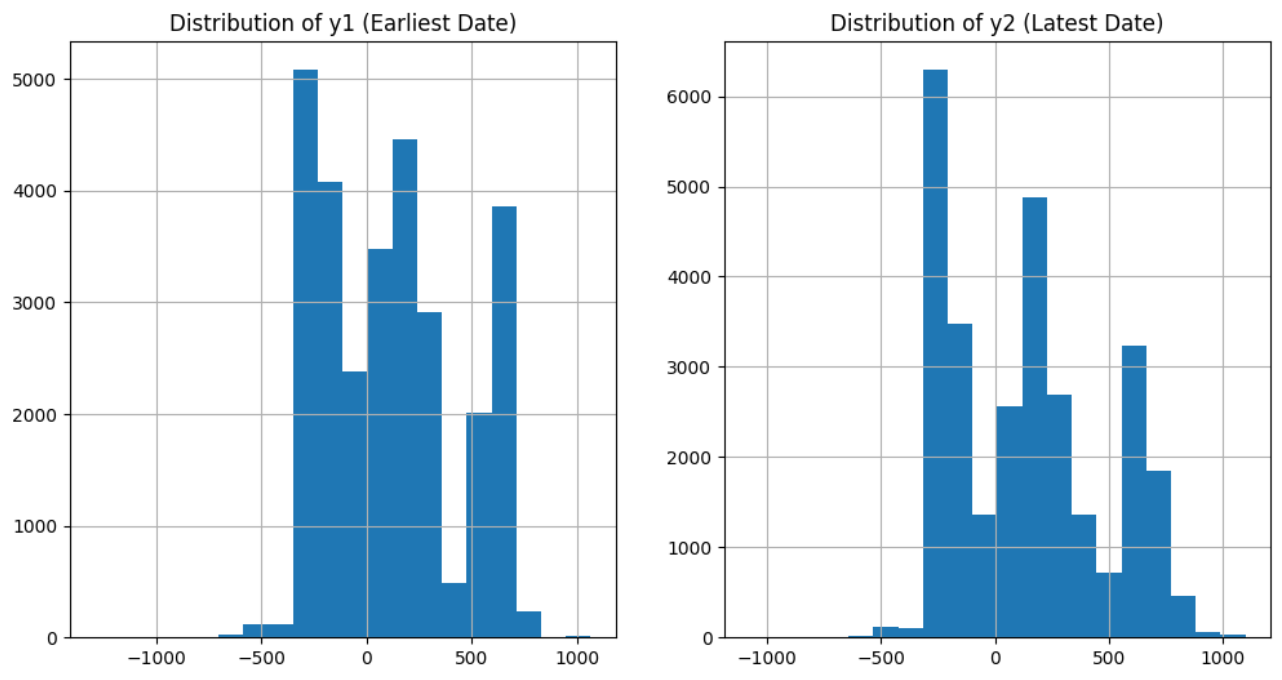
The mean values for the earliest y1 and latest y2 recorded dates were approximately -119 and 146, respectively (see Figure 1 for the distribution of earliest and latest dates).

Figure 1.

Distribution of Earliest Dates (y1) & Distribution of Latest Dates (y2)

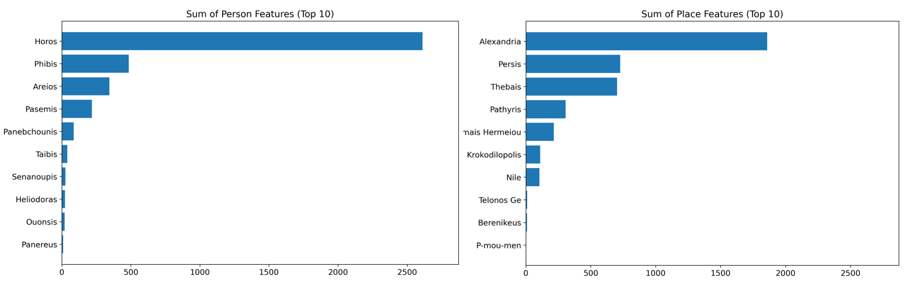
The top 10 most frequently occurring features related to persons and places across the dataset were visualized by generating bar graphs (refer to Figure 2). These visualizations provided insight into key feature distributions and their potential influence on model predictions.

Figure 2.

Figure 2: Top 10 Most Frequently Occurring Features Related to (i) Person & (ii) Place

To determine the most appropriate modeling approach, the distribution of exact (y1 = y2) and non-exact (y1 ̸= y2) year matches in both raw and filtered datasets were assessed. In the raw dataset, it was found 16,698 rows where y1 = y2 and 12,550 rows where y1 ̸= y2. After filtering, the dataset contained 5,239 rows where y1 = y2 and 3,326 rows where y1 ̸= y2. This higher proportion of exact years in both the raw and filtered datasets suggested that regression would be more suitable for the task. It was believed that regression was the better approach because predicting an exact year (a continuous variable) aligns with the strengths of regression, and the majority of the ground truths were a single continuous year rather than a range of years.

Since regression was chosen, a target column that handles both cases: when y1 equals y2 (a single year) and when y1 does not equal y2 (a range of years) was created. The target variable, y target, was set to y1 in cases where the two values were equal. When they differed, the y target was assigned the midpoint of y1 and y2, as the midpoint provides a reasonable estimate for a range when an exact year is unavailable. This new target column replaced y1 and y2 as the ground truth label. All other ground truth labels were dropped, as they were deemed unnecessary for predicting the year a text was written. However, it could be worthwhile to explore using these additional labels as features in the dataset to assess whether they improve model performance.

4.2. Feature Engineering

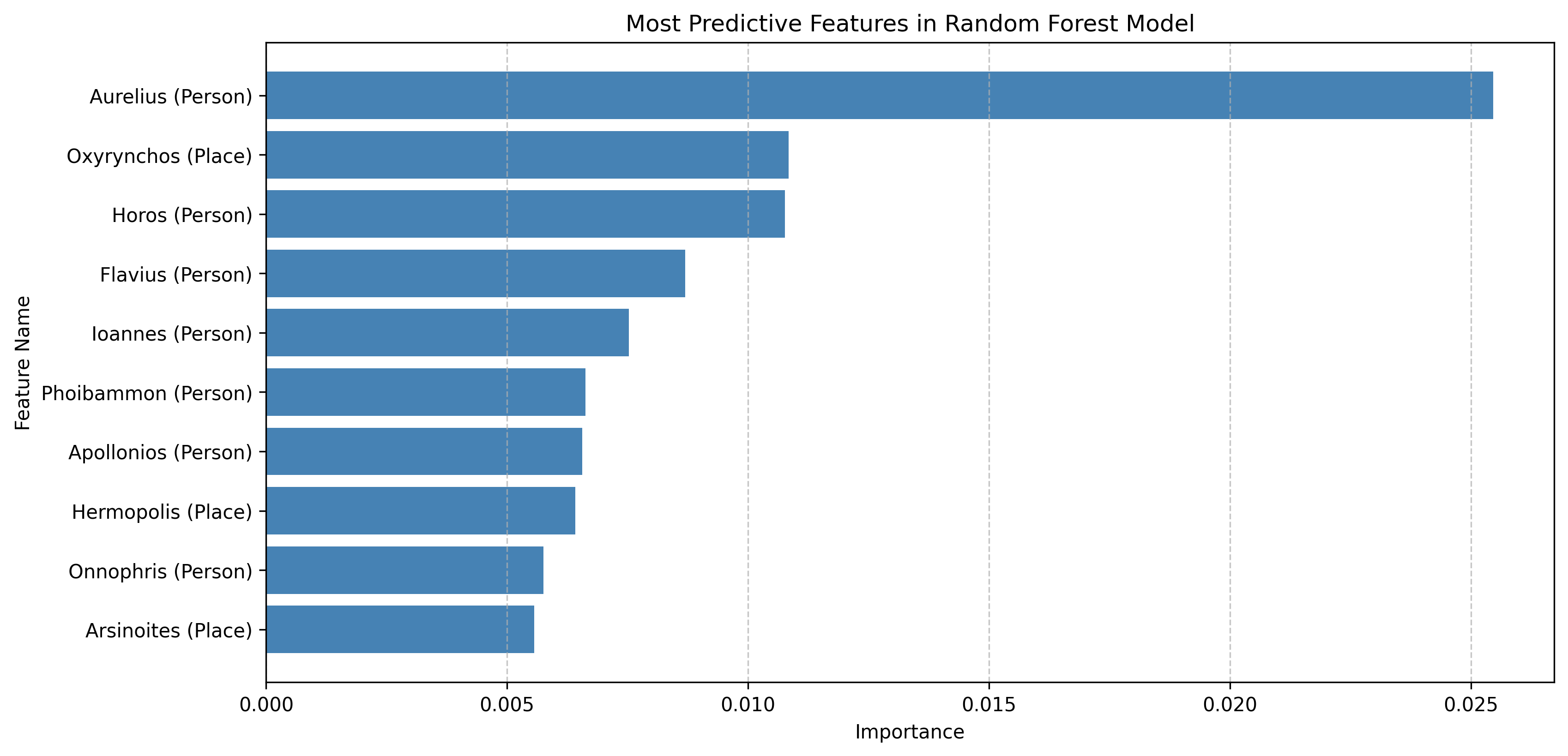
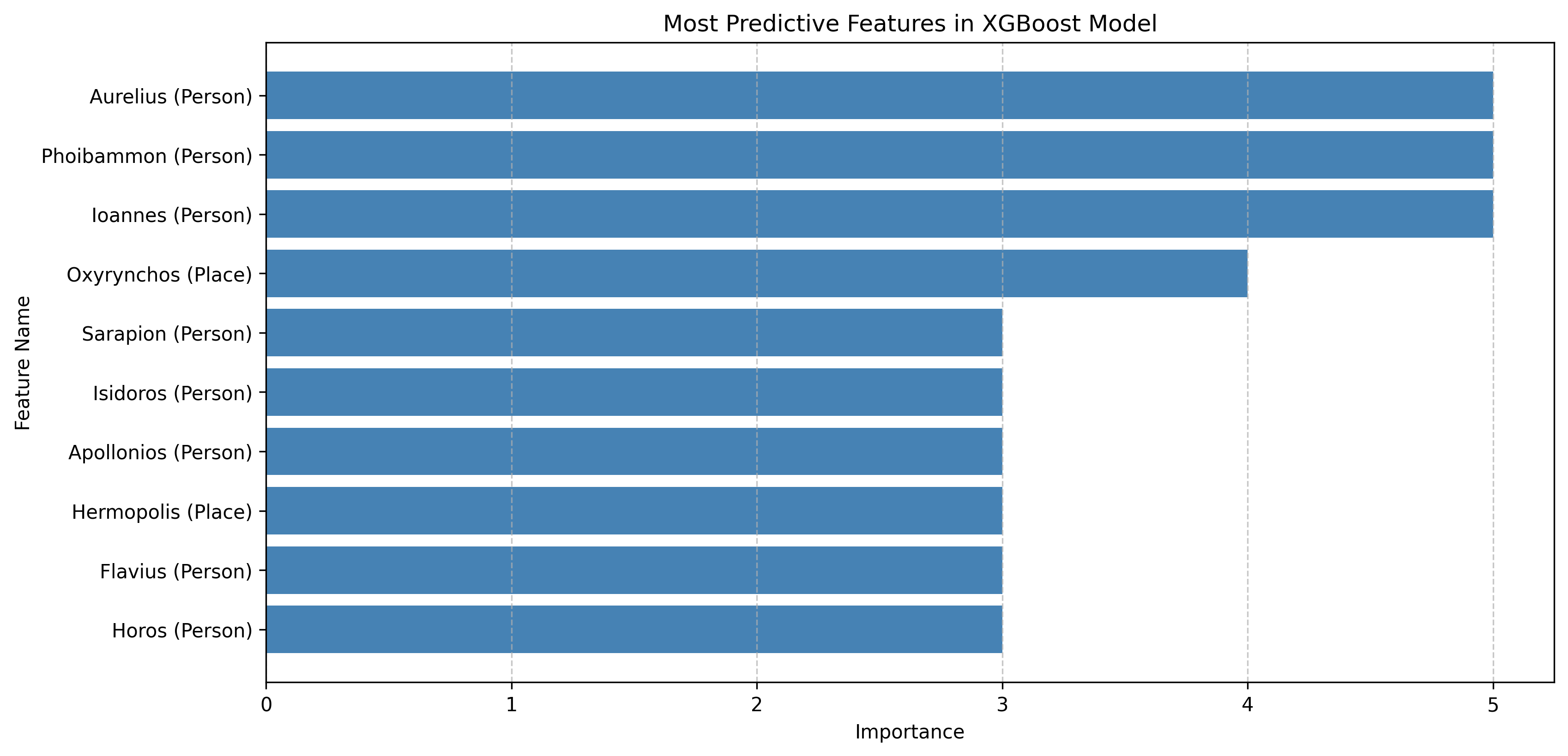
4.2.1. Feature Importance Evaluation

In order to understand the most predictive features, the most predictive Singular Value Decomposition (SVD) transformed features were calculated. Then each singular value decomposition transformed feature was mapped to its original weighted components. Next, the weights were aggregated across all singular value decomposition components to estimate the contribution of each original feature (name/place). The top-ranked features were then selected based on highest weights. The plots below illustrate the top 10 most important features for both the Random Forest and XGBoost models (Figures 3 and 4).

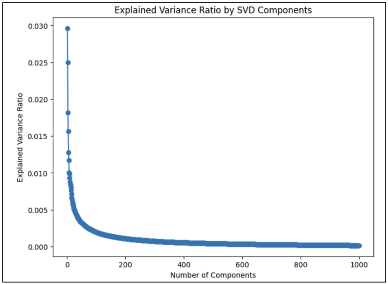
4.2.2. Dimensionality Reduction and Feature Transformation

To address the challenges posed by high-dimensional datasets, singular value decomposition was employed as the method for dimensionality reduction. Singular value decom position is particularly effective in reducing the number of features in sparse matrices, which characterize the dataset. Through empirical testing, 1,000 principal components were selected, allowing for the retention of 95% of the variance in the data despite a reduction in feature count by over 15,000. This choice demonstrated strong performance, as evidenced by the explained variance ratio.

Figure 3.

Top 10 most important features for the Random Forest Model

Figure 4.

Top 10 most important features for the XGBoost model

To better understand the impact of dimensionality reduction through singular value decomposition, an analysis was conducted on the plot depicting the explained variance ratio across the components. This plot illustrates the extent to which the variation in the original data is captured by a specific number of singular value decomposition components (refer to Figure 5).

When exploring the number of components significantly exceeding 1,000, it was observed that variance retention often surpassed 0.9999, leading to suboptimal model performance due to overfitting.

To further refine the dataset, low-variance feature removal was implemented, discarding features with minimal variation across the dataset. The VarianceThreshold was applied to eliminate features with a variance below 0.001, resulting in a reduction of the original 16,383 features to 1,345. This process enhanced computational efficiency while preserving the model’s ability to capture meaningful patterns.

Through the combination of dimensionality reduction with singular value decomposition and low-variance feature removal, a more compact and informative dataset was successfully created. This transformation streamlined the original one-hot encoded features while maintaining key patterns, thereby improving the efficiency and effectiveness of machine learning models.

Figure 5.

Explained Variance Ratio By Singular Value Decomposition Components

4.3. Model Development

4.3.1. Data Preparation and Scaling

To prepare the dataset for model training and evaluation, it was split into training and testing subsets. The features (denoted as (X)) included all input variables, while the labels (denoted as (y)) corresponded to the target years or year ranges for prediction. 80% of the data was allocated for training, while the remaining 20% was designated for testing, and a random seed of 42 was employed to ensure reproducibility during the splitting process.

The purpose of this split was to evaluate the model’s generalization capabilities on unseen data. The training set was utilized to fit the model, while the test set provided an unbiased estimate of its performance.

For most models, scaling was not required due to the dataset being one-hot encoded and subsequently reduced through Variance Thresholding and singular value decomposition. Variance Thresholding eliminated low-variance features without altering their scale, and singular value decomposition produced principal components that were already normalized during the decomposition process. As a result, the features were well-suited for most algorithms without additional preprocessing.

The neural network required additional scaling to ensure efficient and stable training. Given that neural networks are sensitive to feature magnitudes due to their reliance on gradient descent optimization, Feature Scaling and Target Scaling methods were applied.

StandardScaler was applied to (X), transforming each feature to have zero mean and unit variance. This approach mitigated issues such as vanishing or exploding gradients and ensured compatibility with the network’s He Normal weight initialization. In addition, MinMaxScaler was applied to (y), normalizing values to the range [0, 1]. This normalization aligned the target variable with the linear output activation function and the mean absolute error loss function employed during training.

Standardizing the input features improved gradient-based optimization, resulting in faster convergence and more stable weight updates. Moreover, normalizing the target variable ensured that predictions were appropriately scaled to match the training objectives.

After scaling, the final datasets were (X train scaled) and (y train scaled), which was utilized for model training, and (X test scaled) and (y test scaled), which was used for evaluating model performance on unseen data. Scaling transformations were implemented as a pipeline to ensure consistent preprocessing for both training and testing datasets, enhancing reproducibility and reliability.

Additionally, the EarlyStopping callback was utilized during training to terminate the process early if the validation loss ceased to improve. The ReduceLROnPlateau callback was also employed to decrease the learning rate when the model’s performance plateaued. These techniques prevented overfitting, maintaining a validation mean absolute error close to the training mean absolute error (e.g., 49.785 vs. 48).

4.3.2. Model Implementation Ridge

4.3.2.1. Regression

A Ridge regression model was employed with cross-validation using 5 folds. Ridge regression incorporates an L2 regularization term into the linear regression model, penalizing large coefficient values to help prevent overfitting. The strength of the regularization is controlled by the alpha parameter when instantiating the RidgeCV class. The 5-fold cross-validation process involved partitioning the training data into 5 parts, training the model on 4 parts, and validating on the remaining part, repeating this process across all folds.

The mean absolute error, which measures the average absolute difference between predicted values and ground truths, was computed. The best Ridge model yielded a training mean absolute error of 109.62 and a testing mean absolute error of 124.12, representing some of the lowest scores among all models evaluated. The relatively poor performance of Ridge and Lasso regression compared to other models suggested that the data exhibited nonlinear characteristics.

4.3.2.2. Lasso Regression

A Lasso linear regression model was also utilized with 5-fold cross-validation. Lasso regression incorporates an L1 regularization term, allowing some coefficients to be shrunk to zero, effectively reducing the feature set. Despite tuning the alpha hyperparameter, Lasso emerged as one of the poorer performing models, achieving a training mean absolute error of 113.21 and a testing mean absolute error of 125.16 with the optimal alpha value set at 0.109.

4.3.2.3. Random Forest

A Random Forest model was employed for regression tasks, constructing an ensemble of 100 decision trees. This ensemble learning algorithm combines multiple weak decision trees to enhance prediction accuracy and reduce overfitting. Bootstrap sampling was utilized to randomly select samples with replacement from the training data, creating several datasets for training individual trees. Each decision tree predicted a value, and the final prediction was derived from the average of all tree predictions in the forest.

The initial Random Forest model produced significantly better results than the linear models, achieving a training mean absolute error of 30.7 and a testing mean absolute error of 78.6 after 8 minutes and 15 seconds of execution. The Random Forest Regressor emerged as one of the highest-performing models in this study, significantly outperforming linear models such as Lasso and Ridge regression. To further enhance its performance, hyperparameter optimization was conducted using GridSearch with cross-validation, systematically exploring a range of hyperparameter combinations to identify optimal settings for the model.

The parameters tuned included:

max depth: The maximum depth of each decision tree.
min samples split: The minimum number of samples required to split a node.
n estimators: The number of decision trees in the forest. 5-fold cross-validation was employed to ensure the robustness and generalizability of the model during the tuning process.

4.3.2.4. Optimal Hyperparameters

Following the GridSearch process, the following hyperparameters were identified as optimal:

max depth: 20
min samples split: 5
n estimators: 300

4.3.2.5. Model Performance

With the optimized hyperparameters, the Random Forest Regressor was retrained and evaluated on both the training and testing datasets, yielding:

Training Mean Absolute Error: 31.35
Testing Mean Absolute Error: 77.80

The improvements achieved through hyperparameter tuning underscored the model’s ability to capture complex, nonlinear patterns in the dataset. Although the Random Forest Regressor delivered strong results, additional experimentation with other advanced models was conducted to explore further enhancements in predictive performance.

4.3.2.6. Gradient Boosting

The gradient boosting model, specifically XGBoost, was employed as an efficient and accurate framework for machine learning. Various parameters were manually adjusted to improve model performance, reducing the mean absolute error from 81 to 71.

Boosting is an ensemble learning technique that sequentially combines weak learners (such as shallow decision trees) to form a strong learner. Each new tree is trained to correct the errors made by the previous trees. The XGBoost framework incorporates regularization to prevent overfitting, is optimized for speed and low memory usage, and supports sparse data.

The XGBoost model was notably efficient, taking only 20 seconds to run, and achieved a mean absolute error of 71.2 with an R-squared score of 0.84. This R-squared value indicates that 84% of the variation in the target variable was captured by the model, demonstrating the predictive power of the selected features.

4.3.2.7. Neural Network

A deep neural network (DNN) was designed using TensorFlow for regression tasks. The architecture consisted of an input layer that accepted input data with a specified dimension, followed by four hidden layers with progressively decreasing neuron counts to refine feature extraction. The first hidden layer contained 512 neurons with ReLU activation, He initialization, L2 regularization (1e-4), batch normalization, and a dropout rate of 0.36. The second layer had 256 neurons with similar settings but a slightly lower dropout rate of 0.3. The third layer had 128 neurons and followed the same configuration as the second, while the fourth layer contained 64 neurons with reduced L2 regularization (1e-5). The final output layer consisted of a single neuron with a linear activation function, making it suitable for regression tasks.

To optimize performance and prevent overfitting, batch normalization was incorporated after each hidden layer, facilitating faster convergence and reducing sensitivity to initialization. The Adam optimizer with gradient clipping was utilized to enhance stability during training. The model was trained with a learning rate of 1e-2, a batch size of 512, and for a total of 500 epochs. Early stopping was applied, monitoring validation loss with a patience of 50 epochs, while learning rate reduction halved the rate after 8 epochs without improvement, with a minimum learning rate of 5e-7. Key hyperparameters, including learning rate, batch size, and early stopping patience, were fine-tuned based on validation performance.

To further optimize the model, several techniques were implemented:

Dropout Regularization: Prevents over-reliance on specific neurons by randomly dropping units during training.
Learning Rate Scheduling: The ReduceLROnPlateau callback was implemented to halve the learning rate after 8 epochs without improvement.
Early Stopping: Training was halted when validation loss plateaued, ensuring computational efficiency.
10-Fold Cross-Validation: The model was evaluated across 10 folds to minimize bias and variance.

4.3.2.8. Ensemble Models

Finally, individual model outputs were combined using weighted ensemble techniques, which included:

Weighted Neural Network Ensemble: The neural network ensemble was constructed by leveraging the models generated during 10-fold cross-validation. Each of the 10 neural network models which were trained on a unique combination of training and validation splits, was preserved. These models were then combined into a single ensemble by computing a weighted average of their predictions. The weights were determined based on each model’s validation performance, assigning greater influence to models with lower mean absolute error. By aggregating models trained on distinct training-validation splits, the ensemble incorporated diverse learned patterns, which reduced model bias and variance, leading to stronger generalization. As a result, the neural network ensemble achieved a lower mean absolute error than any individual model, highlighting the benefit of aggregating multiple individually trained models into a stronger predictive model.
Super Ensemble: Integrated outputs from the neural network, Random Forest, XGBoost, and LightGBM models. Although this approach did not achieve the lowest mean absolute error, it demonstrated the potential for blending diverse algorithms to capture varied aspects of the data.

The super ensemble served as an experimental approach to validate the robustness of the combined methodologies, balancing trade-offs between mean absolute error and R-squared scores.

4.3.3. Hyperparameter Tuning

Hyperparameter tuning was performed for different models based on their respective characteristics using methods such as LassoCV, RidgeCV and GridSearchCV for the RandomForest model. LassoCV and RidgeCV are specialized implementations of the Lasso and Ridge regression in scikit-learn that automatically optimize the alpha parameter through cross validation. Similarly, GridSearchCV enables an exhaustive cross validation search over a predefined set of hyperparameter values to identify the optimal configuration.

For the Lasso and Ridge regression models, the alpha hyperparameter was tuned, as it determines the strength of regularization applied to the model’s coefficients. Optimizing alpha is crucial to balancing bias and variance, thereby preventing both underfitting and overfitting. Hard-coded alpha values were specified for the RidgeCV model to evaluate its performance across different levels of penalization.

For the Random Forest model, hyperparameters were optimized, including n estimators (number of trees), max depth (maximum depth of each tree), and min samples split (minimum number of trees required to split a node). Using GridSearchCV, predefined values for these hyperparameters were explored to determine the optimal combination. Once the best hyperparameters were identified, the RandomForestRegressor was trained with the optimized settings, leading to expected performance improvements.

Further exploration of other models was conducted to assess potential improvements in predictive performance. The Gradient Boosting model underwent manual hyperparameter tuning, where parameters were adjusted iteratively based on the mean absolute error of each model iteration. The tuned parameters included colsample_bytree, learning_rate, max_depth, alpha, and n_estimators, to determine the configuration that minimized the mean absolute error. If a change in a hyperparameter value resulted in a lower mean absolute error, further adjustments were made in the same direction until the improvement plateaued. Once a parameter reached an optimal value, the next hyperparameter was tuned following the same approach. This iterative process was repeated until no further reductions in mean absolute error were observed, ensuring that the model achieved the best possible performance with the tuning constraints.

Initial results from the Support Vector Machine (SVM) model indicated poor performance, with a mean absolute error of 226.18. However, visualizing predictions against actual values revealed that the predictions were clustered around 100, suggesting the need for hyperparameter adjustment. Increasing the C hyperparameter to 956.1 improved the support vector machine’s mean absolute error to 94.5.

For the neural network model, key hyperparameters, including learning rate, batch size, and number of epochs, were fine-tuned to enhance predictive accuracy. A dynamic learning rate was implemented using the ReduceLROnPlateau callback, which halved the learning rate, whenever validation loss plateaued for 8 epochs. A batch size of 512 was selected to balance training speed and accuracy, as smaller batch sizes improved accuracy but extended training time, whereas larger batch sizes reduced accuracy while accelerating training. Additionally, early stopping was employed to prevent overfitting and unnecessary training.

Following these optimizations, the neural network model achieved an average mean absolute error of 49.785 with a standard deviation of 3.87, demonstrating significant improvement over the initial configurations. This tuning process emphasized the importance of hyperparameter optimization in refining model performance and highlighted the value of cross-validation in ensuring robust and reliable results.

4.4 Evaluation

To prepare the dataset for model training and evaluation, it was split into training and testing subsets. 80% of the data was allocated for training and 20% for testing, using a random seed of 42 to maintain reproducibility. The feature matrix x comprised all input variables, while the target variable y represented the predicted year or year ranges.

4.4.1. Cross-Validation

Cross-validation was employed to enhance the robustness of model performance and mitigate the risk of overfitting. For Lasso linear regression and Ridge regression, a 5-fold cross validation approach was utilized. In the case of the Random Forest regressor, GridSearch cross-validation was implemented, as discussed in Section 4.3.2, “Model Implementation.”

For the neural network model, to ensure robust performance and prevent overfitting, 10-fold cross-validation was implemented. This method allows for the assessment of model robustness.

10-fold cross-validation was performed for the NN model with k set to 10, resulting in the dataset being divided into 10 equal subsets. For each fold, the model was trained on 9 of the subsets and validated on the remaining one, ensuring that each subset was utilized for validation exactly once.

The main steps in the cross-validation process are outlined as follows:

Model	Mean Absolute Error
Lasso	124.89
Ridge	123.8
Random Forest	77.8
XGBoost	71.4
Support Vector Machine (SVM)	94.53
Neural Network (NN)	48
RF + XG + LGBM + NN Ensemble	47
Weighted Neural Network Ensemble	45.7
Super Ensemble (Everything)	46.9

Table 1.

Mean Absolute Error values for various models

Data Splitting: The dataset was divided into 10 equal subsets. Within each fold, feature scaling was performed using StandardScaler, while target values were scaled using MinMaxScaler.
Model Training and Evaluation: For each fold, a new model was instantiated using a neural network function create model (see section 4.3.2), which defined a neural network architecture comprising four dense layers, dropout layers, batch normalization, and L2 regularization. The model was compiled with the Adam optimizer, utilizing a learning rate of 1e-4, and trained on the training subset. The validation subset was employed to evaluate the model’s performance.
Metrics: Model performance was assessed using the mean absolute error metric, which served as a key evaluation criterion for the regression task. The mean absolute error was computed for the validation fold, and the average mean absolute error across all folds was recorded.

Upon completion of the cross-validation process, the model exhibiting the lowest average validation mean absolute error was selected for further evaluation and testing, thereby ensuring that the model’s hyperparameters were optimized for generalization.

4.4.2. Metrics

4.4.2.1. Mean Absolute Error

Mean Absolute Error is utilized to quantify the average magnitude of errors in a set of predictions, without considering their direction. The mean absolute error values for various models are presented in Table 1.

The best overall model in terms of mean absolute error was the Weighted Neural Network Ensemble (see section 6.1), which achieved the lowest test mean absolute error of 45.7.

4.4.2.2. R-Squared (R²)

R-squared (R²) is a statistical measure that represents the proportion of variance for a dependent variable that’s explained by an independent variable or variables in a regression model. The R² values for the models are summarized in Table 2.

Model	R²
Lasso	0.62
Ridge	0.62
Random Forest	0.80
XGBoost	0.84
Neural Network (NN)	0.867
RF + XG + LGBM + NN Ensemble	0.9277 (Highest)
Weighted Neural Network Ensemble	0.8878
Super Ensemble (Everything)	0.89

Table 2.

R² values for the models

The best overall model for R² was determined to be the RF + XG + LGBM + NN

Ensemble, exhibiting a high R² value closest to 1.

5. Results

Results from the analysis of historical text dating using various machine learning models reveal that the relationships within the dataset are predominantly nonlinear. The results clearly demonstrate the dataset’s nonlinearity, as linear models like Lasso and Ridge Regression performed poorly, with mean absolute error values exceeding 120 years, failing to capture complex temporal patterns. In contrast, nonlinear models such as Random Forest, XGBoost, and Neural Networks significantly reduced mean absolute error (as low as 45.7) and achieved higher R² scores, confirming their ability to model intricate relationships between named entities and historical time periods. The findings highlight the importance of leveraging various nonlinear machine learning techniques, such as ensemble models (Random Forest, XGBoost, LightGBM) and deep learning (Neural Networks), capable of capturing complex interactions in the data. This insight significantly influenced the model selection process, highlighting the necessity of employing advanced methods capable of capturing these complex interactions.

Linear models, such as Lasso and Ridge Regression, demonstrated inferior performance compared to their nonlinear counterparts. The results reinforced the notion that the underlying data exhibits intricate relationships that linear models cannot effectively capture.

Ensemble methods like Random Forest and XGBoost, exhibited superior performance in identifying complex patterns within the data.

The implementation of a neural network model further capitalized on the nonlinear nature of the data. This approach allowed the exploration of deep learning techniques, which are well-suited for capturing complex relationships. The neural network achieved competitive performance, demonstrating its adaptability to the dataset’s intricacies.

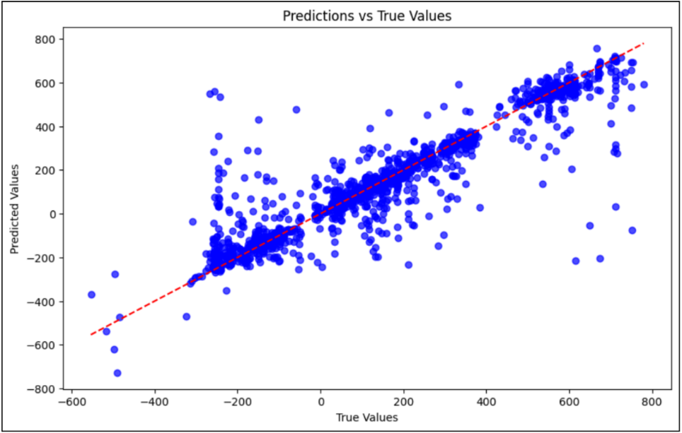
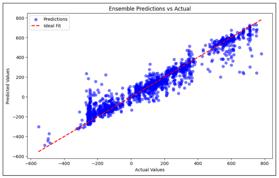
5.1. Visual Metrics

Scatter plots comparing predicted values to actual for each model (see example Figures 6 and 7) revealed two distinct periods (200 BC and within the range of 600-700 AD) where the predictions deviated from the actual values. The scatter plots exhibit a high dispersion of points, particularly in earlier historical points, which suggests unique challenges, such as limited training data or ambiguous named entities in these periods. Further refinement of the feature set or the inclusion of additional historical context may be necessary to enhance predictions for these challenging periods.

Figure 6.

Actual vs. Predicted Years - Neural Network

Figure 6:

Figure 7.

Actual vs. Predicted Years - 10-Fold Ensemble

5.2. Selected Examples

Here we present a selected set of examples to demonstrate the usage of this method. The table contains three of the best predictions (lowest error) and three of the worst predictions (highest error), along with the most influential features that led to the prediction (the positive values next to the feature indicate that there is a positive association between the existence of that feature and the prediction. The negative value indicates that there is a negative association between the existence of that feature and the prediction.

Case	Actual	Predicted	Abs Error	Influential Features
Best #1	248.0	248.0	0.0	Alexandros (+0.5), Lykophron (0.4), Oaphres (-0.4), Ammonios (+0.3)
Best #2	120.0	120.1	0.1	Herakleides (+0.4), Aurelia (-0.3), Arsinoe (-0.2)
Best #3	15.0	15.1	0.1	Apollonios (+0.5), Gorgias (-0.3), Kallias (-0.3)
Worst #1	-256.0	184.2	440.2	Demetrios (+0.6), Isidoros (-0.4), Horion (-0.4), Karanis (-0.3)
Worst #2	-120.0	300.4	420.4	Philoxenos (+0.5), Tryphon (-0.4), Theon (-0.3)
Worst #3	-80.0	310.2	390.2	Sarapis (+0.5), Dionysia (-0.3), Paniskos (-0.3)

Table 3.

Top 3 best and worst model predictions with influential features.

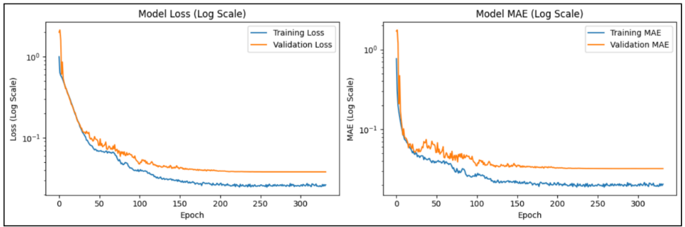
Figure 8 shows the neural network’s training and validation loss (left) and mean absolute error (right) over epochs on a logarithmic scale. Model loss stabilized within the 150-200 epoch range.

Figure 8.

Figure 8: Training and validation loss over epochs (log scale) and Training and validation mean absolute error over epochs (log scale)

6. Discussion

This study showcases machine learning, especially ensemble models, for dating historical texts, offering a scalable approach for computational humanities.

6.1. Performance of Different Models

The evaluation of multiple models revealed that linear models such as Lasso and Ridge Regression performed poorly, with high mean absolute error values exceeding 120 years. These models assume a linear relationship between features and the target variable, which does not align with the inherent complexities of historical text data.

In contrast, nonlinear models outperformed their linear counterparts, with Random Forest achieving a test mean absolute error of 77.8, while XGBoost further improved it to 71.4. The success of tree-based models indicates that named entities (person and

place names) contain nontrivial temporal signals that can be effectively captured through decision tree splits.

The deep learning approach using a neural network produced an even lower mean absolute error of 48, confirming that neural networks can model intricate data structures more effectively than traditional methods. Notably, the 10-fold cross-validation on the neural network yielded a similar mean absolute error of 49.78, indicating that the model generalizes well across different data subsets.

Finally, among the ensemble models evaluated, the 10-Fold Ensemble, which is the weighted average of predictions from all neural network 10-fold models that optimized overall regression performance, achieved the lowest mean absolute error of 45.7, indicating its superior accuracy in minimizing prediction errors (Table 1).

However, the RF + XG + LGBM + NN Ensemble demonstrated the highest R² value of 0.9277 (see Table 1 and Table 2), signifying its ability to explain the largest proportion of variance in the target variable (predicted year of authorship) while still maintaining a competitive mean absolute error of 47. Although the 10-Fold Ensemble slightly outperforms in terms of absolute error, the RF + XG + LGBM + NN Ensemble provides a strong balance between accuracy and predictive power, making it the best overall model for historical text dating.

6.2. Cross-Validation and Generalization

The study highlights the importance of cross-validation in ensuring model generalization. Lasso and Ridge regression models were evaluated using 5-fold cross-validation, while Random Forest underwent 5-fold cross-validation with hyperparameter tuning via GridSearch. The use of cross-validation helped mitigate overfitting and provided a more reliable estimate of model performance. In contrast, the SVM and XGBoost models were optimized using manual hyperparameter tuning. The ensemble models, which combined multiple predictions, were evaluated using weighted averaging techniques to leverage the strengths of individual models while minimizing their weaknesses.

The results from cross-validation further validate the importance of nonlinear models for this task. The neural network model achieved an average mean absolute error of 49.78 across its 10 validation folds, demonstrating its ability to generalize well to unseen data. The Random Forest model also benefited from cross-validation through hyperparameter tuning with GridSearch, leading to optimized results with improved generalization performance.

6.3. Importance of Model Selection in Historical Text Dating

A key insight from this study is the necessity of choosing models that align with the dataset’s structure. The poor performance of linear models underscores the presence of nontrivial patterns in historical text data. The significant improvement achieved by nonlinear models such as XGBoost and Random Forest highlights the importance of ensemble learning in predicting authorship dates. These models reduced the mean absolute error from over 120 years (Lasso and Ridge) to around 71 for XGBoost and 77 for Random Forest.

The best performing models were the ensemble approaches, which combined Random Forest, XGBoost, LightGBM, and Neural Network. The 10-Fold Ensemble model (refer to section 6.1) achieved the lowest mean absolute error of 45.7 years, confirming that ensemble learning is beneficial for capturing the complex relationships within historical text data.

6.4. Future work

As the current model relies primarily on named entities, which limits the scope of information used for predictions, future work could incorporate additional features such as text metadata, stylistic elements, or linguistic analysis to better capture cultural and historical context. Incorporating features related to language style, sentence structure, or thematic elements could provide a richer dataset, leading to more accurate predictions.

While nonlinear models performed well, further improvements could be achieved through more extensive hyperparameter tuning. Techniques such as grid search, random search, or Bayesian optimization could refine model parameters and enhance predictive accuracy. Additionally, exploring different neural network architectures, activation functions, and training strategies may reveal more optimal solutions. Future research could also integrate probabilistic modeling techniques or deep learning approaches that could provide a more nuanced way to manage date uncertainty, offering confidence intervals rather than single-year predictions.

Moreover, the lack of cross-validation for support vector machine and XGBoost suggests that further evaluation using systematic validation methods could enhance reliability, particularly in cases where performance varied across historical periods.

By refining and expanding this computational approach, this research advances the field of digital humanities and historical text analysis. The ability to date historical texts with greater accuracy and efficiency offers scholars and archivists a powerful tool for preserving and understanding historical narratives. With continued improvements in feature engineering, modeling techniques, and dataset expansion, machine learning-based approaches have the potential to revolutionize historical manuscript dating and related fields.

7. Conclusion

This study developed a machine learning regression model to predict the authorship dates of historical texts using named entities, specifically person and place names, as temporal markers. Unlike traditional historical manuscript dating methods, which rely on physical examination, paleographic analysis, or expert interpretation, this approach introduces a scalable and non-destructive alternative capable of efficiently processing large textual datasets. The key contribution of this work is the demonstration that named entities can serve as effective temporal indicators, providing a novel feature set for dating historical texts. By structuring the dataset as a one-hot encoded matrix of named entities and implementing regression techniques, this study introduces a computational framework that refines the estimation of textual origins.

The results highlight that the model performs well in predicting exact years for texts where definitive dates are available. Linear models such as Lasso and Ridge Regression struggled to capture the complexities of the data, resulting in poor performance. In contrast, nonlinear models, including Random Forest and XGBoost, significantly outperformed linear methods by effectively modeling intricate patterns. To further enhance predictive accuracy, deep learning approaches using neural networks were explored, demonstrating competitive performance and scalability for larger datasets. Among all models tested, the ensemble approach proved to be the most effective, capturing the most variance and achieving the highest predictive accuracy. With a mean absolute error of 45.75 years, the 10-fold ensemble (refer to section 6.1) model successfully estimated authorship dates within a reasonable margin, demonstrating its potential for historical text dating.

Challenges arose when dealing with texts containing anachronistic references or names persisting across long historical spans, leading to occasional misclassifications. Additionally, while this approach demonstrated reasonable predictive accuracy, some degree of error persisted, particularly for texts with limited historical context or insufficient named entity occurrences.

Despite these promising findings, several areas for improvement remain. The assumption that named entities alone are reliable indicators of time is not always valid, as historical figures and locations can appear in texts written long after their referenced period. Furthermore, the accuracy of historical name annotations in the dataset directly impacts model performance, introducing potential noise. Handling texts with uncertain date ranges also presents an ongoing challenge, requiring further methodological refinement to account for temporal ambiguity.

The modeling approach used in this study, using text-derived features to date historical texts, can be applied broadly across digital humanities datasets. Many humanities corpora share structural similarities: They contain named entities, locations, chronological indicators, and stylistic patterns that vary across authors, regions, or time periods. Models like the one used here can help uncover latent structure within these features, enabling researchers to detect authorship signals, identify regional or administrative variations, trace linguistic change, or predict missing metadata such as date, provenance, or genre. Because the framework is feature-centric and interpretable, it is well-suited for historical corpora where transparency and scholarly justification are essential. Therefore, similar workflows could support research in areas such as epigraphy, manuscript studies, or historical newspaper analysis, allowing scholars to systematically explore patterns that are difficult to see through manual inspection alone.

Works Cited

Assael et al. 2025 Assael, Y., Sommerschield, T., Cooley, A., Shillingford, B., Pavlopoulos, J., Suresh, P., Herms, B., Grayston, J., et al. (2025) “Contextualizing ancient texts with generative neural networks”, Nature, 645(8079), pp. 141–147. Available at: https://doi.org/10.1038/s41586-025-09292-5.

Broux and Depauw 2015 Broux, Y., and Depauw, M. (2015) “Developing onomastic gazetteers and prosopographies for the ancient world through named entity recognition and graph visualization: Some examples from trismegistos people”, in L. Aiello and D. McFarland (eds.) Social Informatics. SocInfo 2014. Lecture Notes in Computer Science (Vol. 8852). Springer, Cham.

Castro et al. 2004 Castro, K., Vandenabeele, P., Rodríguez-Laso, M., Moens, L., De Schryver, S., and Van Hooydonk, G. (2004) “Micro-raman analysis of coloured lithographs”, Analytical and Bioanalytical Chemistry, 379(5-6), pp. 674–683.

Depauw 2018 Depauw, M. (2018) “Trismegistos. optimizing interoperability for texts from the ancient world”, in A. De Santis and I. Rossi (eds.) Crossing Experiences in Digital Epigraphy. From Practice to Discipline. De Gruyter, pp. 191–199.

Depauw and Van Beek 2009 Depauw, M., and Van Beek, B. (2009) “People in Greek documentary papyri. First results of a research project”, The Journal of Juristic Papyrology, 39, pp. 31–47.

Dhali et al. 2020 Dhali, M.A., Jansen, C.N., de Wit, J.W., and Schomaker, L. (2020) “Feature-extraction methods for historical manuscript dating based on writing style development”, Pattern Recognition Letters, 131, pp. 413-420. Available at: https://www.sciencedirect.com/science/article/pii/S0167865520300386.

Hamid et al. 2018 Hamid, A., Bibi, M., Siddiqi, I., and Moetesum, M. (2018) “Historical manuscript dating using textural measures”, in 2018 International Conference on Frontiers of Information Technology (FIT), pp. 235-240.

Han et al. 2023 PLACEHOLDER

He et al. 2014 He, S., Sammara, P., Burgers, J., and Schomaker, L. (2014) “Towards style-based dating of historical documents”, in 2014 14th International Conference on Frontiers in Handwriting Recognition, pp. 265-270.

Hellwig 2019 Hellwig, O. (2019) “Dating Sanskrit texts using linguistic features and neural networks”, Indogermanische Forschungen, 121, pp. 1-27.

Jull et al. 1995 Jull, A.J.T., Donahue, D.J., Broshi, M., and Tov, E. (1995) “Radiocarbon dating of scrolls and linen fragments from the Judean desert”, Radiocarbon, 37(1), pp. 11–19.

Koopmans et al. 2024 Koopmans, L., Dhali, M.A., and Schomaker, L. (2024) “Performance analysis of handwritten text augmentation on style-based dating of historical documents”, SN COMPUT. SCI., 5(397). Available at: https://doi.org/10.1007/s42979-024-02688-6.

Kumar et al. 2011 Kumar, A., Lease, M., and Baldridge, J. (2011) “Supervised language modeling for temporal resolution of texts”, in Proceedings of the 20th ACM International Conference on Information and Knowledge Management. New York, NY, USA: Association for Computing Machinery, pp. 2069–2072. Available at: https://doi.org/10.1145/2063576.2063892.

Moscato et al. 2022 Moscato, V., Craig, H., Haque,M.N., Huang, K., Sloan, J., and Corrales de Oliveira, J. (2022) “Multiple regression techniques for modelling dates of first performances of Shakespeare-era plays”, Expert Systems With Applications, 200, 116903. Available at: https://doi.org/10.1016/j.eswa.2022.116903

Omayio et al. 2022 Omayio, E.O., Indu, S., and Panda, J. (2022) “Historical manuscript dating: Traditional and current trends”, Multimedia Tools and Applications, 81, pp. 31573–31602. Available at: https://doi.org/10.1007/s11042-022-12927-8

Pavlopoulos et al. 2024 Pavlopoulos, J., Konstantinidou, M., Marthot-Santaniello, I., Essler, H., and Paparigopoulou, A. (2024) “Dating Greek papyri with text regression”, in Proceedings of the 61st Annual Meeting of the Association for Computational Linguistics. Toronto, Canada: Association for Computational Linguistics, pp. 1–12. Available at: https://doi.org/10.18653/v1/2023.acl-long.556

Ren et al. 2023 Ren, H., Wang, H., Zhao, Y., and Ren, Y. (2023) “Time-aware language modeling for historical text dating”, in H. Bouamor, J. Pino, and K. Bali (eds.) Findings of the Association for Computational Linguistics: EMNLP 2023. Singapore: Association for Computational Linguistics, pp. 13646–13656. Available at: https://aclanthology.org/2023.findings-emnlp.911/.

Ullah and Jamjoom 2022 Ullah, Z., and Jamjoom, M. (2022) “An intelligent approach for Arabic handwritten letter recognition using convolutional neural network”, PeerJ Computer Science, 8, e995. Available at: https://doi.org/10.7717/peerj-cs.995.

Van Schaik 2013 Van Schaik, S. (2013) “Dating early Tibetan manuscripts: A paleographical method”, Scribes, Texts and Rituals in Early Tibet and Dunhuang, pp. 119–135.

Wahlberg et al. 2016 Wahlberg, F., Wilkinson, T., and Brun, A. (2016) “Historical manuscript production date estimation using deep convolutional neural networks”, in 2016 15th International Conference on Frontiers in Handwriting Recognition (ICFHR), pp. 205-210. Available at: https://doi.org/10.1109/ICFHR.2016.0048

Yu and Huangfu 2019 Yu, X., and Huangfu, W. (2019) “A machine learning model for the dating of ancient Chinese texts”, in 2019 International Conference on Asian Language Processing (IALP), pp. 115-120. Available at: https://doi.org/10.1109/IALP48816.2019.9037653

This work is licensed under a Creative Commons Attribution-NoDerivatives 4.0 International License.

URL: https://dhq.digitalhumanities.org/editorial/000831/000831.html
Comments:
Published by: and
Affiliated with: Digital Scholarship in the Humanities
DHQ has been made possible in part by the National Endowment for the Humanities.
© 2025 the authors

Unless otherwise noted, the DHQ web site and all DHQ published content are published under a Creative Commons Attribution-NoDerivatives 4.0 International License. Individual articles may carry a more permissive license, as described in the footer for the individual article, and in the article’s metadata.