Abstract
The Voynich Manuscript (VM) is a medieval manuscript likely written in the 15th
century (Yale Univ., Beinecke Rare Book & Manuscript Library MS 408).[1] The manuscript is written in an unknown language or code using an
unidentified set of symbols that has yet to be made legible. Additionally, the
codex contains many strange and fantastical images of plants, people, and
cosmological/zodiac illustrations, the meaning of which are also unknown. One of
the main research avenues into the VM is to examine its textual content to
understand how it behaves relative to known texts; this can provide insight as
to whether the mysterious writings contain decipherable text or not. In this
paper, we explore the coherence and flow of the manuscript using Latent Semantic
Analysis (LSA). LSA is a technique that may help ascertain whether the behavior
of the text within the VM shows evidence of a coherent flow of topical content,
by comparative analysis of text samples that are near each other, farther away
from each other, at section breaks, or even page breaks. The advantage of this
strategy is that LSA analysis can be undertaken without actually knowing the
meaning of the text. We expect portions of text that are near to each other to
have a relatively high similarity score, that is, to be potentially semantically
related. We also expect that at anticipated topic breaks (pages or sections),
the similarity score between adjacent text blocks would be smaller, as the
breaks seem to represent a change in topic. Both of these patterns are observed
in the control manuscript studied as proof-of-concept experiments. Patterns then
observed in several sections of the VM suggest that there may be an overall
coherence to the text.
1. Introduction
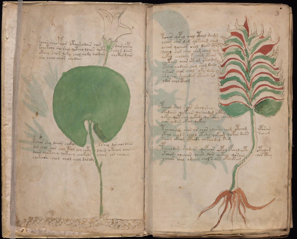
The Voynich Manuscript has been called The World's Most Mysterious Manuscript
[
Manly 1921], and for good reason. On the one hand, the
Voynich Manuscript (VM) is a typical medieval manuscript written and decorated
using iron-gall ink and natural pigments, on parchment that has been
carbon-dated to the early fifteenth century (ca. 1420). Nothing mysterious about
that. But upon opening the codex, the utterly unique features of this intriguing
object become immediately apparent. The manuscript is written entirely in an
otherwise-unattested set of symbols (known as Voynichese) and illustrated with
unidentifiable plants, uninterpretable astrological diagrams, and astonishing
biological drawings. The Voynich Manuscript has intrigued, mystified, and
frustrated linguists, cryptologists, enthusiasts, and scholars worldwide for
centuries. This essay presents a novel approach to the still-unanswered question
of whether the manuscript has underlying meaning at all.
For the present study, it is important to understand the structure of the
manuscript. Examining the manuscript’s physical structure reveals that the
visual transitions that seem to indicate new topics are also structural
transitions. These visual transitions (for example, from a series of
illustrations of plants to a series of what appear to be cosmological diagrams)
occur at physical breaks between
“quires,” the gatherings of
nested folded sheets of parchment. The illustrative sections, scribes,
languages, and structure of the manuscript are summarized in Table 1. In the
Quire Structure column, the baseline Arabic numerals represent the sequential
numbering of the quires, while the superscript numerals indicate how many leaves
are in each quire. For example,
“28-1” means that Quire 2 originally had eight leaves (four
nested bifolia) but is lacking one, and
“3-78” means that Quires 3 through 7 each
have eight leaves. The table below also indicates which of the five scribes
identified in [
Davis 2020] contributed to each section and which
variant type of
“Voynichese” is used in each section (
“Language A” or
“Language B,”
as first identified and described in [
Currier 1976]). It should
be noted additionally that Scribe 1 writes in
“Language
A,” while the other four scribes consistently use
“Language B.” These distinctions will be discussed
further below.
| Section |
Scribe(s) |
Languages |
Quire Structure |
| Botanical (ff. 1r-66v) |
1, 2, 3, 5 |
A, B |
18, 28-1
(lacking f. 12), 3-78, 810-6 (lacking ff. 59-64) |
| Cosmological/Astronomical/ Astrological diagrams (ff. 67r-74v) |
4 |
B |
9-112 , 122-1
(lacking f. 74) |
| Biological (ff. 75r-84v) |
2 |
B |
1310 |
| Rose foldout (ff. 85r-86v) |
2, 4 |
B |
141 (a single large sheet) |
| Pharmaceutical/Recipes (ff. 87r-102v) |
1, 3 |
A, B |
154, [16: lacking], 178-4 (lacking ff. 91-92, 97-98), [18:
lacking], 194
|
| Stars (ff. 103r-116r)[1]
|
3, 2 |
B |
2014-2 (lacking ff. 109-110) |
Table 1.
Summary of the Voynich Manuscript
In spite of these visually coherent sections, even after a century
of study we still do not know whether the manuscript demonstrates
textual coherence. Do the various sections represent a coherent
whole, or are they unrelated to one another? Does the text within each section
demonstrate internal coherence? Such questions have important implications for
“reading” the manuscript. In a textbook, for example,
topics discussed in a particular chapter will, by and large, be related to one
another and will inherently have some sort of semantic similarity, as a single
overarching topic is being addressed. We would expect that the closer two pieces
of text are to one another, on average, the higher their similarity, as it is
more likely the topics being presented would be closely related. By extension,
we expect that the flow or coherence of the text would diminish at a chapter
break, as the topic is likely to change. Using techniques such as Latent
Semantic Analysis (LSA) we can measure the similarity between two blocks of text
(called “documents” below), analyzing relationships between a
set of documents and their constituent words (called “terms”
below); it is particularly useful for revealing hidden (latent) semantic
structures in textual data (rather than semantic meaning) and determining if
those relationships hold (for technical details about LSA, see Appendix 1). By
applying the LSA technique to known texts (as baselines) and to the unknown text
of the Voynich Manuscript, we can address the question of coherence in the VM.
If the analysis of the Voynich Manuscript suggests some degree of coherence and
flow, this may suggest that there is indeed a coherent message underlying the
mysterious text. It is important to keep in mind that we are not making a claim
about reading or deciphering the Voynich Manuscript; LSA analytics functions by
identifying patterns and context, not semantic meaning.
2. Latent Semantic Analysis
The technique employed in these experiments is known as Latent Semantic Analysis
(LSA) [
Deerwester et al. 1990], a technique that originated in the field
of Information Retrieval (IR). The methodology analyzes sets of documents
(paragraphs, articles, emails or other writing) to determine how similar they
are to each other. In a given text or texts, it is quite likely that a variety
of words will be used to express similar ideas or concepts. For example, there
might be a paragraph about cars, one about vehicles, and a third that focuses on
automobiles. Human readers know they are related, but a computer will treat the
distinct words as separate entities. LSA is a method that identifies these
hidden (i.e.
“latent”) underlying structures and
relationships between the words in these documents by analysing the patterns of
word usage across the compared texts. In essence, because words that appear
together in similar contexts tend to have similar meanings, LSA considers which
words occur in which documents, finds patterns relating to how these words
co-occur with one another, and uses those findings to infer underlying
relationships or concepts. Two compared documents that share these
relationships/concepts will tend to return a high similarity score.
A full mathematical explanation of LSA can be found in Appendix 1 in addition to
a discussion of its strengths/weaknesses and parameter decisions that were made
for the present study.
[2] We will provide a brief
high-level description here. For a given manuscript, such as the Voynich, we
partition it into smaller
“documents” approximating a set
size (say 20, 30 or 40 terms) after performing some pre-processing on the text.
An \(n\) by \(m\) matrix \(A\) (where \(n\) corresponds to the number of unique terms
and \(m\) corresponds to the number of
documents) is formed from these documents such that each row is a term, each
column corresponds to a document, and each cell in the matrix, say \(A_{ij}\), corresponds
to a Term
Frequency (TF) count where \(A_{ij}\) represents the number of times term \(i\) occurs
in document \(j\). This representation is known
as a
Bag-of-Words (BoW) model, in which each document is simply a
collection of terms and the order of the terms is not taken into account. LSA
takes into account which terms occur together (as in the same document) or are
used in similar ways and does not use additional positional context of the
terms. Further modification of these values may take place in order to scale
them to achieve better results.
[3]
This \(A\) matrix is then
transformed using a Singular Value Decomposition (SVD) which, in essence,
creates new vectors representing our documents which we can then use in
computations to generate similarity scores between them. These new document
vectors bring out the underlying
“latent” features and
relationships between the terms and documents by reducing the noise in the data.
We refer to this transformation of \(A\) as our
“semantic space” representing the
collection of processed documents.
In order to compare the similarity of two documents, we calculate the cosine
between their vectors (akin to columns in \(A\)); the higher the cosine, the greater
the similarity. The
cosine score is based on the angle between the two vectors. Vectors with a
smaller angle between them (generally those that “point” in
the same general direction) have a higher cosine and therefore a higher
similarity than those that present a larger angle and a smaller cosine. With a
known text such as the Aberdeen Bestiary (discussed
below), we generally interpret this as semantic similarity, because two compared
documents, if they have a high similarity score, are likely to be discussing a
similar subject or theme. We can confirm this by referring back to the original
text. With the Voynich, such referential confirmation is not possible, as we do
not know for certain whether or not the Voynich contains semantically meaningful
content. In the case of the Voynich, then, this analysis is a measurement of the
latent similarity of term usage within and across visually coherent sections.
Although we cannot know, until such time as the manuscript is rendered legible,
whether these connections are truly semantic or not, we can
ascertain whether or not the Voynich Manuscript behaves in a similar way to
known texts. This may be viewed as evidence that 1) there is in fact semantic
content within the manuscript, and 2) visually coherent sections are also
textually coherent.
It is worth taking a moment to explain why we believe LSA to be a valid
methodology in this case. LSA is a 35-year-old IR technique that has largely
fallen out of use in favour of new and more modern Natural Language Processing
(NLP) approaches. Because of the unique nature of the Voynich manuscript,
however, LSA has great potential. Within the Voynich are only about 35,000
terms. More modern techniques such as Word2Vec [
Mikolov et al. 2013] and
Transformers [
Vaswani et al. 2017] generally rely on document sets in
the order of millions or billions (or far more when we consider the cutting edge
LLMs like ChatGPT, Gemini, or Grok) in order to generate reliable results.
Because the dataset size for the Voynich is much too small for popular modern
techniques, we are forced to go back to more
“old school” NLP
methodologies. LSA has been demonstrated to work well with datasets of this
size; for example [
Dos Santos and Favero 2015] used a semantic space of only
359 documents to perform automated evaluation of students’ written answers.
Latent Semantic Analysis is therefore a natural choice to analyze the coherence
and flow of the Voynich Manuscript.
2.1. Previous Related Works
There are several published experiments that support the choice of LSA for
this project. [
Foltz, Kintsch, and Landauer 1998] conducted an experiment to
demonstrate an approach for predicting the coherence of sets of texts by
manipulating textual coherence and assessing readers’ comprehension. One
takeaway from this work was the creation of an automated methodology that
can generate coherence predictions. [
Foltz, Kintsch, and Landauer 1998] utilized LSA
as a technique for measuring the semantic relationship between two given
pieces of text. The first experiment they performed involved four versions
of a textbook. A 300-dimension semantic space was created using the first
2,000 characters of each of the 30,473 articles from Grolier’s Academic
American Encyclopedia (details of this can be found in [
Landauer and Dumais 1997]). The metric they used was an analysis
of adjacent sentence-by-sentence comparisons using LSA, and a calculation of
the average cosine. The original coherence score (i.e. average cosines) was
0.192 and was improved to 0.403 in the final version. Another experiment
they performed was to detect discourse segmentation, attempting to identify
points in the text where a topic shift occurs (thus enabling the
segmentation of the text into distinct topics). The idea behind this is
based on the hypothesis that coherence scores should be lower between the
portions of the text where the discourse topics change. To test this idea,
they used the methodology to predict the breaks between nineteen chapters of
an introductory psychology textbook. They created an LSA semantic space for
the textbook by partitioning it into paragraphs and created a dataset from
which a semantic space of 300 dimensions utilising 4,903 paragraphs by
19,160 unique terms (some paragraphs were removed in pre-processing as they
represented references, problem sets, and other components that were not
relevant to the discourse). To smooth the predictions, a sliding window of
10 paragraphs was utilized. Two adjacent blocks of ten paragraphs were
compared using the cosine operator, after which the window would be advanced
by one paragraph. This was repeated over all the paragraphs in the text. The
average cosine over the entire text was 0.43 while the average cosine
between paragraphs across chapter breaks was only 0.16, a result that was
statistically significant. By selecting coherence breaks that were two
standard deviations below the mean they successfully identified nine of
eighteen chapter transitions. As the cutoff point was increased, more breaks
were identified but so, too, were false positives, which increased at a
linear rate. Some of the chapter breaks with unexpectedly higher scores
(0.25 and 0.29) were found to comprise text that linked the two chapters,
accounting for these higher values that are still, it should be noted, well
below the mean of 0.41.
[
Timm and Schinner 2023] performed several experiments on the
Voynich Manuscript in order to ascertain how related or unrelated the
Currier
“Language A” and
“Language B” variants might be. They utilized a vector space
model built from the Voynich Manuscript where documents are created from
individual pages. These pages are represented by vectors utilising the Term
Frequency (TF) of each term present on the page (so the vectors will consist
mostly of zeroes — this is analogous to the columns in the \(A\) matrix described
earlier).
They concluded there is no sudden transition between the two
“languages”, A and B, and that there is a gradual
evolution between them after experimenting with cosine calculations between
all possible pairs of pages. One possible drawback to the Timm &
Schinner approach is their reliance on the TF model of the text. A cosine
will only score a non-zero value if there is text overlap between the two
documents being compared. While valuable, the TF approach does not identify
underlying latent relationships, structure, or synonymy. By contrast, LSA
has the advantage of recognising and scoring relationships between words,
identifying relationships between non-identical words that may be
functioning synonymously. Additionally, TF values can skew results because
terms that are very common can artificially inflate the similarity scores.
Weighting methods such as Term Frequency-Inverse Document Frequency (TF-IDF)
and Log-Entropy
[4] can help smooth out these discrepancies.
[
Reddy and Knight 2011] performed a similar page-wise comparison
experiment on the Voynich Manuscript that focused on whether or not it was
likely the leaves of the manuscript are in the correct order. Like [
Timm and Schinner 2023], they created a TF vector for each page
and performed page-wise comparisons using the cosine operator, results which
suffer from the same weaknesses outlined above. They published results of
page comparisons with the pages
“scrambled” in which the
scrambled adjacent-page similarity scores were close to 0, while they showed
higher similarity when pages were scored in accordance with the manuscript’s
current page sequence. They do, however, note that some of the
non-contiguity of the herbal/pharmaceutical sections and the A/B language
distinctions may suggest that some pages were probably re-ordered.
[
Sterneck, Polish, and Bowern 2021] investigated topic modelling in the Voynich
Manuscript using techniques such as Latent Dirichlet Allocation (LDA),
Latent Semantic Analysis (LSA) and Nonnegative Matrix Factorization (NMF).
The objective was to try and cluster the text in the Voynich to look for any
interesting clusters of subjects or topics. This included using features
such as Lisa Fagin Davis’s five scribal corpora, A/B language
classification, visual subject label (astrology, botanical, balneological,
rosette, recipes/starred section and unknown), and individual quires. The
text was vectorized on a page by page basis (with TF-IDF weighting applied
to the NMF/LSA methods to increase the visibility of rare words and decrease
the influence of words that are quite common) and fed into the cluster
algorithms after being transformed by one of the previously mentioned
methods (LDA/LSA/NMF) and introducing a dimensionality reduction phase
(reducing the high-dimensional space created by these methods into a
lower-dimensional space that may enable topics or concepts to be more
visible in the analysis). The k-means clustering algorithm was then utilised
and results presented. Initial results were generated using all three
methods, but additional experiments were continued using only NMF; this was
due to identified issues with LDA (picking optimal parameters) and potential
issues with LSA, a technique that does not perform well with polysemy or
homophony as such relationships dilute the method’s ability to discover
underlying latent connections between word usage. Entropy experiments in
[
Lindemann and Bowern 2021] suggest this may be an issue,
although our experiments either did not encounter these issues or found them
to be negligible, if present at all. Based on their experiments (largely
using NMF), Lindemann and Bowern suggest the text in the Voynich Manuscript
likely represents an enciphered human language rather than
“meaningless” text and that the illustrative topics
can be clustered to some degree.
3. Methodology
The framework of the experiments conducted here is based on the research by [
Foltz, Kintsch, and Landauer 1998] which was briefly highlighted in the previous
section. Specifically, we will use their method for determining document
coherence as well as performing discourse segmentation on the Voynich Manuscript
and a select known text.
The coherence experiment is fairly straightforward in principle. Given a semantic
space for a particular text, we consider all the adjacent columns in the
\(D^T\) matrix. The columns,
from 1 to \(m\) (where \(m\) is the number of documents) are
in the same order in which they were processed from the original text. That is,
column \(j\) and \(j+1\) are adjacent in the original
text. To perform a coherence measurement, we simply take the cosine scores
between all the adjacent documents from 1 to \(m\) the pairs (1, 2), (2, 3), …, (\(j\)
\(j+1\)), …, (\(m-1\), \(m\)). The average of these scores is then
calculated, and we treat that as the coherence score. A second set of
calculations is performed by taking a permutation of the order of the documents
that are compared such that no two adjacent documents are present in the
permutation and comparison scores (and the average) is once again calculated.
This is done 10 times for the random permutations, and an overall average is
calculated. The two values can then be compared. It is expected that the average
for the correct-order documents is significantly higher than the average for
random permutations.
For each dataset used in the coherence experiment, a number of semantic spaces
will be created. These will use documents of approximately 20, 30 and 40 terms,
each which will be represented in the semantic space as individual columns in
\(D^T\). Additionally,
before the creation of the semantic space via the SVD operation, the \(A\) matrices
will be weighted using
TF, TF-IDF and Log-Entropy weightings. Each text will therefore have a total of
nine semantic spaces generated for the experiment to allow for comparison
between them. The comparison mechanism (using a document of, say, size 30) for
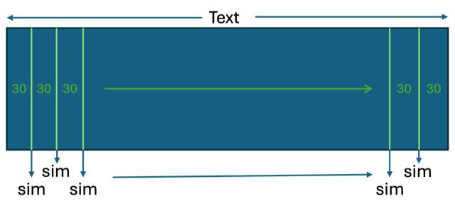
the coherence scores can be seen conceptually in Figure 2. The similarity score
is the cosine value of the two vectors representing the documents from the
semantic space.
With the discourse segmentation experiment, we can test the ability of the
methodology to identify significant features such as section breaks, chapter
breaks, page breaks, or other transitions. This experiment uses the Voynich
Manuscript and one known text (the Latin
Speculum Humanae
Salvationis
[5]) so we can
compare the behaviours between them. If we can detect semantically-significant
features in the known text, then it may indicate that similar features or
behaviors in the Voynich suggest some sort of semantic structure.
For this experiment, the data sets were partitioned into logical sections: For
the
Speculum we used chapters and for the Voynich
we used pages. Within each Voynich page, paragraph, circular text, and radial
text were grouped separately for further partitioning into documents (because we
do not know whether these different formats serve different functions within the
manuscript). We then generated documents from these partitions of approximately
size 20 and size 40
[6]. The
size 40 documents, utilizing TF-IDF weighting as per the previous experiment,
were used for creation of the LSA semantic space; the size 20 documents were
utilized in the discourse segmentation experiment explained below.
The documents created for the discourse segmentation comparisons were windows of
10 concatenated documents from those generated of size 20 (for VM pages with
sparse text, the concatenated “documents” were obliged to
span more than one page). These concatenated documents were used for
side-by-side comparisons in sliding windows. The larger concatenated documents
functioned to reduce the variance between comparisons and create a smoother
picture of the flow of the discourse, as well as detecting when changes may be
occurring.
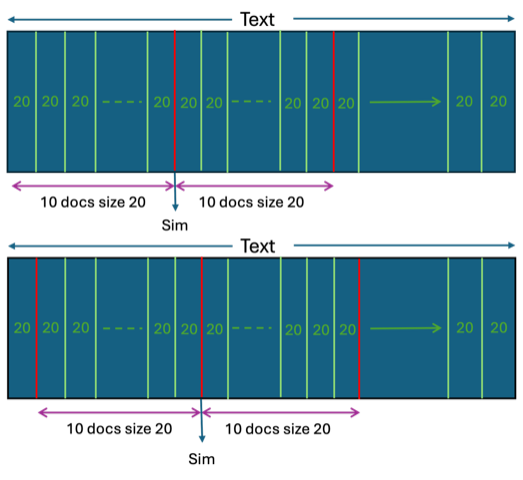
The moving window of textblocks is illustrated in Figure 3, showing the
comparison of two concatenated documents (of 10 x 20 each). The next comparison
is made by sliding each of these concatenated documents over by one document,
resulting in the introduction of new text (and overlap with the previous
comparison). This is repeated until we have exhausted all the text windows.
An example of this step is given below. For the Voynich the first two 10 X 20
documents are represented as:
1r-1,1r-2,1r-3,1r-4,1r-5,1r-6,1r-7,1v-1,1v-2,1v-3[ — ]
2r-1,2r-2,2r-3,2r-4,2v-1,2v-2,3r-1,3r-2,3r-3,3r-4
In this example,
1r-1 is the first document of 20 terms on f. 1r, 1r-2 is the second document of
20 on f. 1r, and so on. The window moves to 1v-1 after all of the 1r text has
been segmented. 1v-3 is the tenth and final document of this window. The symbol
[ — ] represents the transition from one group of ten to the next. The
concatenated document to be compared begins with 2r-1 and proceeds by groups of
20 until the tenth, which is the fourth document on f. 3r. The next comparison
would shift the window by one segment, beginning with 1r-2 and ending with 3v-1:
1r-2,1r-3,1r-4,1r-5,1r-6,1r-7,1v-1,1v-2,1v-3,2r-1[ — ]
2r-2,2r-3,2r-4,2v-1,2v-2,3r-1,3r-2,3r-3,3r-4,3v-1
The process
continues until the last window advances to the end of the text. Each similarity
score is recorded, paying particular attention to page, section and scribal
changes.
3.1 Datasets
For the initial coherence experiments, we employed several open-access texts
in addition to the VM. These texts were chosen because they represent a
variety of linguistic and stylistic genres: George Orwell’s
Animal Farm (approachable contemporary English
prose in a coherent narrative); The
Aberdeen
Bestiary (didactic and formal medieval Latin and a modern
English translation, with each chapter representing a different and
clearly-defined topic)
[7]; Dante’s Inferno (rich and poetic medieval Italian in a
chapter-based narrative); the
Speculum Humanae
Salvationis (didactic and formal medieval Latin in
topically-varied chapters), and computer-readable Voynichese generated via
the software
[8] kindly provided by Torsten Timm [
Timm and Schinner 2020]
[9]. For the VM ASCII transcription, we
used ZLversion 2a dated 17/03/2022, which is the most complete, consistent,
and accurate transcription available.
[10] The wide variety of chosen texts should prove useful to demonstrate
the coherence measurement and the behaviour of the texts in these contexts.
We would expect them all to behave in a somewhat similar fashion regardless
of the style of the writing. The artificial text generated via the Tim and
Schinner (2020) algorithm is meant to mimic the Voynich Manuscript text,
according to their self-citation hoax hypothesis, and preserves some of its
statistical features (for example, the generated text should follow Zipf’s
law). Their hoax hypothesis states that the text gradually changes over time
based on various observations they have made on the manuscript (that many
words in close proximity with one another are also very similar to one
another — for example Voynich terms such as
qokeedy and
qokeey. Although we can’t use this to generate every
section of the Voynich Manuscript individually, we used it to create a set
of text roughly the same size as the Voynich. The algorithm only simulates a
subset of the manuscript text and there is no language A/B distinction (they
do not subscribe to the fact that there is anything really significant
between them and it is a natural function of this gradual shift in
text/words over time that causes it); in their experiments they generated a
portion of text of roughly the same size as recipes section in the
manuscript.
Before we can utilize LSA, there are several steps that must be undertaken to
prepare each text for further use. These steps are typical for the
application of many NLP algorithms, such as lowercasing or removing
punctuation and stop words. As the VM cannot be
“lowercased” (since it has no identifiable upper- or
lower-case characters), we pre-processed all of the baseline texts in other
ways for consistency: removing punctuation and using an algorithm to
tentatively identify and remove the stop words. Stop words are common terms
that, due to their grammatical function and frequency, offer very little
value to the semantic discourse. In practice, stop words act as background
noise that can dilute other relationships in the text. In English these are
words such as “the”, “of”, “is”, etc. Again, in order to
treat all of the texts consistently, stop words were determined for all
texts using an automated method, detailed in Appendix 1. Because we do not
know what the stop words are in the Voynich Manuscript, we used the same
algorithm for all of the texts instead of referring to pre-existent lists of
stop words in the relevant languages. This gives us a like-for-like basis of
comparison.
The VM ZL Transliteration file underwent additional pre-processing. The file
follows the Intermediate Voynich MS Transliteration File Format (IVTFF)
version 1.7 as defined in (Zandbergen, IVTFF - Intermediate Voynich MS
Transliteration File Format - File Format 1.7 2020) that categorizes the
text present in the VM. Voynichese “words” (terms) are
generally classified based on their graphic context: In the IVTFF
transliteration, each term is tagged as occurring in a standard paragraph,
standing alone as a “label,” or written in a non-standard
layout such as around a circle or radiating from a central hub. Our analyses
typically disregard “labels” as they offer little to the
discourse and more than 50% of them are hapax
legomena (terms that only occur once in the text).
“Paragraph” texts behave in ways that are similar to
the legible texts in our comparison datasets and thus are most useful for
LSA analytics. We also removed any terms from the VM transliteration that
are tagged as uncertain in any way, such as terms with unclear spacing or
ambiguous characters.
Table 2 presents statistics for the processed texts, including total word
count, size of stop word list, word count after stop-word
removal/pre-processing and the total number of hapax
legomena (unique words) in the text. Note that it is the total
terms after stop word removal that are used for document segmentation as
well as construction of the semantic space although in practice hapax terms
are not considered in similarity comparisons scores, as they only occur once
and the SVD operation therefore has no context for comparison.
| Text |
Language |
Total Words |
Stop Words (SW) |
Total After SW Removal |
Hapax Legomena |
| Animal Farm |
English |
30,023 |
31 |
18,360 |
2,228 |
| Aberdeen Bestiary |
English |
71,001 |
47 |
38,886 |
4,221 |
| Aberdeen Bestiary |
Latin |
45,109 |
17 |
37,236 |
9,407 |
| Dante’s Inferno |
Medieval Italian |
32,383 |
18 |
24,164 |
4,642 |
| Speculum Humanae Salvationis (Vincent of Beauvais) |
Latin |
40,224 |
17 |
33,773 |
6,677 |
| Voynich Generated |
Artificial |
31,950 |
27 |
19,636 |
1,265 |
| Voynich – ZL |
? |
31,955 |
25 |
24,324 |
4,802 |
Table 2: Post-Processing Text Statistics for Coherence Test Data
4. Results
The results for both the coherence and the discourse segmentation experiments are
reported below, followed by discussion and analysis of these results.
4.1 Coherence Experiment
For each LSA semantic space, we compared the first document (of size 20, 30
or 40) to its adjacent document in order to calculate a similarity score; we
repeated the experiment by shuffling the sequence of compared documents such
that no two consecutive documents were compared. Since shuffling them is a
stochastic process, this was repeated 10 times, and an average of the ten
scores was calculated. In other words, we ran the two tests on each of the
seven textual datasets: one by calculating the average similarity of
adjacent documents, and another using a shuffled set of documents. For each
of the text samples, nine semantic spaces were created by applying three
weighting methodologies (TF, TF-IDF, Log-Entropy) to three different
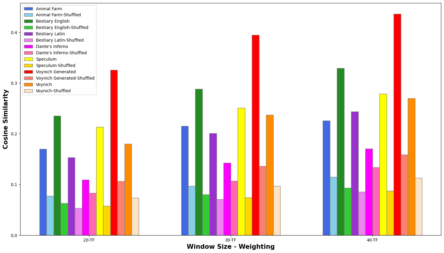
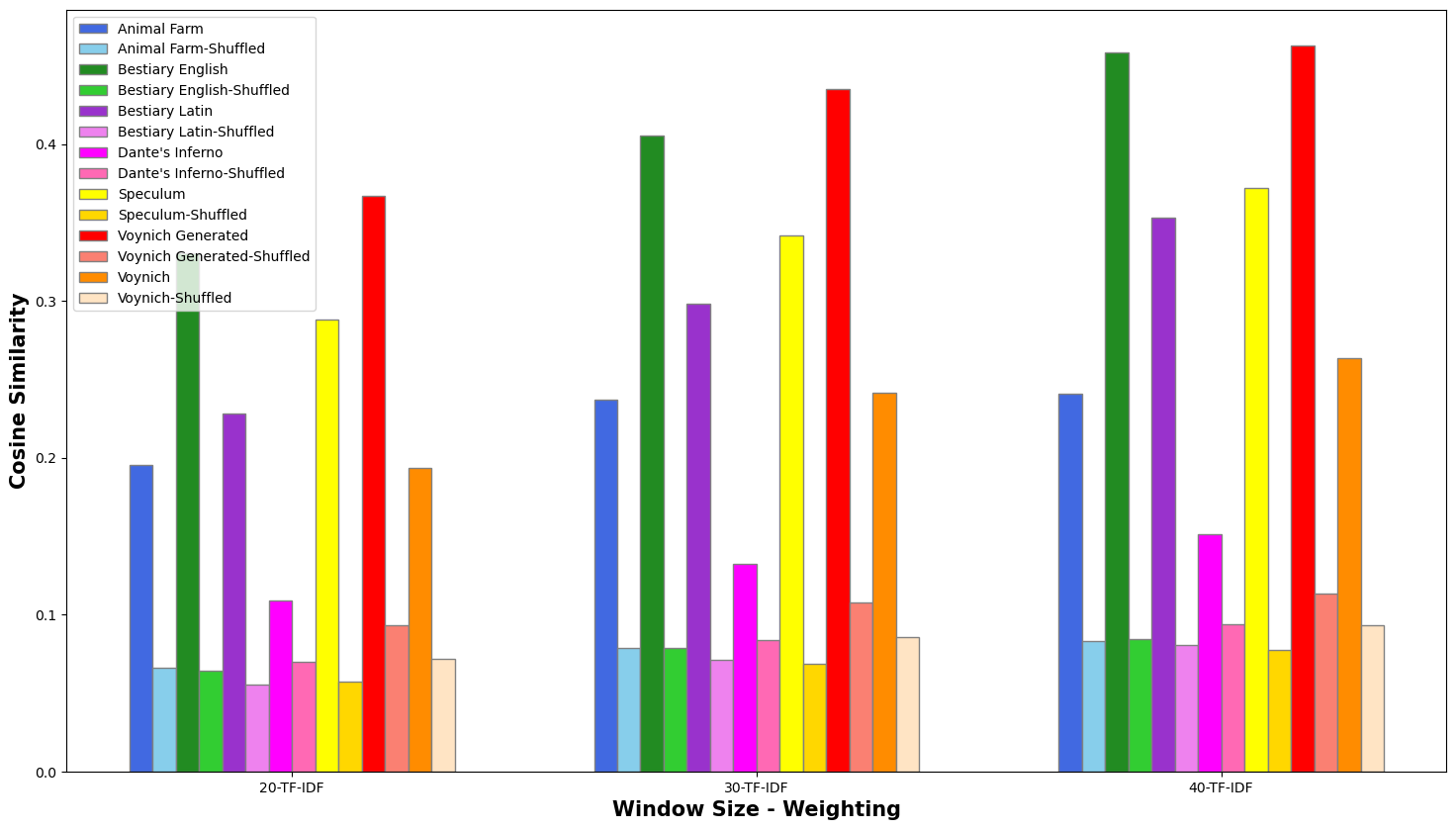
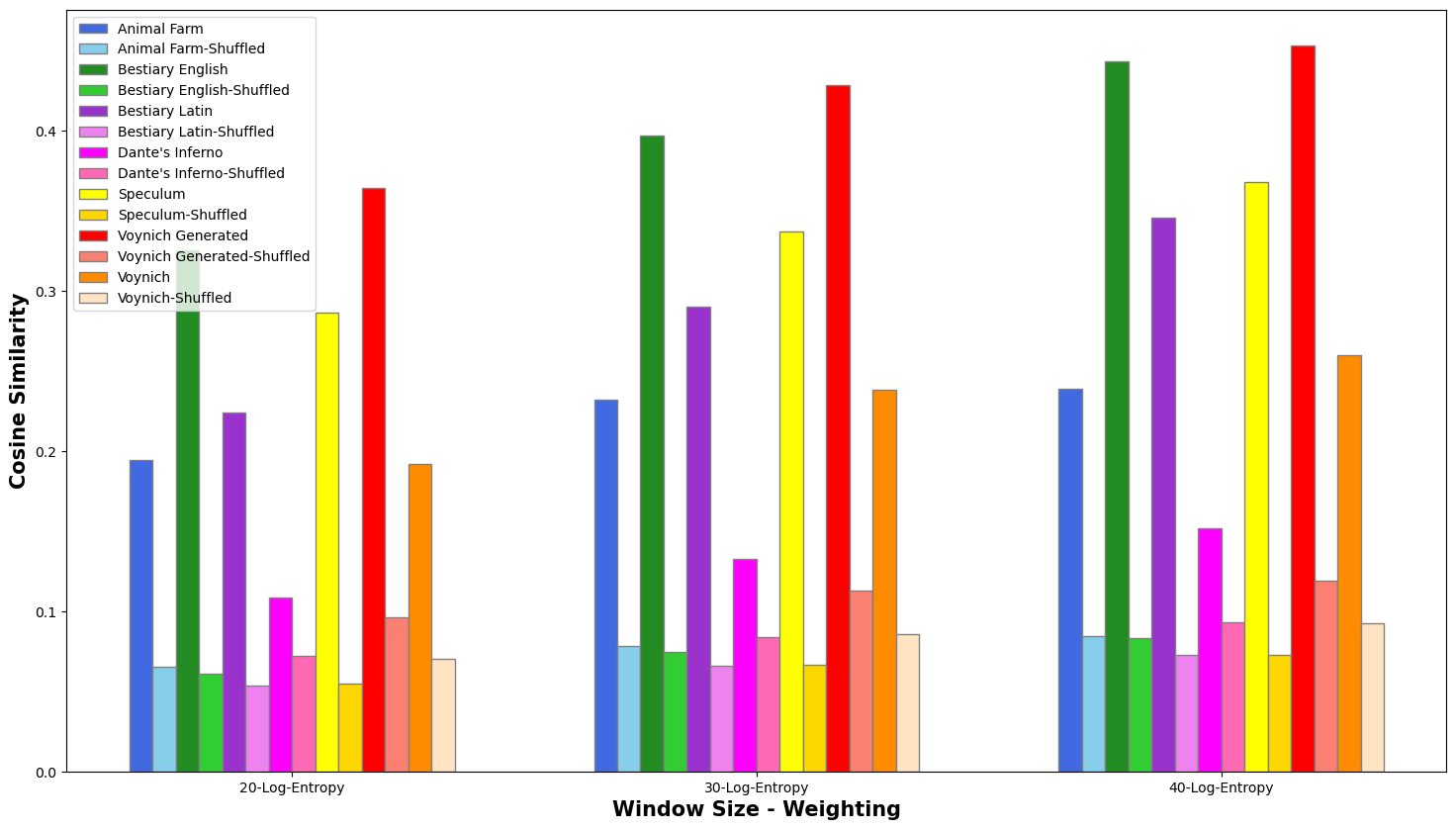
document sizes (20, 30, 40). The results (i.e. the average similarity score
across the entire text) are reported in Figures 4-6:
In each case, the average similarity for the in-sequence text was
significantly higher than the shuffled-text results, demonstrating that the
method correctly responds to adjacency vs. non-adjacency. The TF weighting
(Figure 4) gave the lowest scores, while TF-IDF and Log-Entropy produce very
similar results. The LSA semantic space of 40 resulted in the most visible
contrast between “correct” and shuffled texts. For this
reason, we used documents of (approximately) size 40 using TF-IDF for the
discourse segmentation component of our experiments. The charts demonstrate
that the results on known texts are in line with what would be expected.
Additional statistical tests were performed to determine if the results were
statistically significant. The Shapiro-Wilk test and D’Agostino’s K0 squared
test were performed on the cosine values to determine if the raw similarity
score distribution was normal; this was negative in all cases. We performed
the Mann-Whitney U to test for significance. All of the comparisons scored
well below a \(p\) value of
0.05 — in fact most were close to zero with the highest \(p\) value recorded being
0.000145. In other words, the results were indeed statistically
significant.
4.2 Discourse Segmentation Experiment
The experiments above demonstrated that the text in the Voynich Manuscript
behaves as would be expected for a meaningful text. In the following
experiments, we will test the ability of a methodology called “discourse segmentation” to identify significant
features such as section breaks, chapter breaks, page breaks, or other
transitions, using the Speculum as a
proof-of-concept text. A successful experiment would indicate that the same
method might be able to detect similar features in the Voynich Manuscript.
We first applied this to the known text, the
Speculum. This was done on two versions of the
Speculum. We used both the original
Speculum and a ‘cleaned’ version (removing clauses
that do not contribute to the semantic reading of the text such as the words
“Chapter 1” or the summaries of the previous
chapter that begin each new one). This is in line with the work done by [
Foltz, Kintsch, and Landauer 1998], the source of this technique. For the unaltered
Speculum dataset, the average similarity
score across the entire text was 0.440 and the average score at chapter
breaks was significantly lower, 0.225. This shows a clear distinction
between the complete text and the chapter breaks overall. Using the cleaned
version of the
Speculum, the results show
slightly more contrast, with a higher overall average of 0.445 and a lower
average score at chapter breaks of .212. This indicates that removing the
small amount of redundant text at the beginning of each chapter allowed for
a more accurate comparison of the actual content of each chapter. It should
be noted at this point that all further results reported using the
Speculum dataset use this ‘cleaned’ version.
We used the bottom 5% of the results as a cutoff point for
investigation.
[11] Can characteristics of
the compared text samples explain the low scores? Are the compared documents
truly dissimilar, or are they false negatives? In these explanations, we
will reference a generic concatenated document of size twenty as
d1-d2-…-d9-d10 [ — ] d11-d12 …-d19-d20, where
“dx” is a document, and [ — ] represents the transition from one
cluster of ten to the compared group.
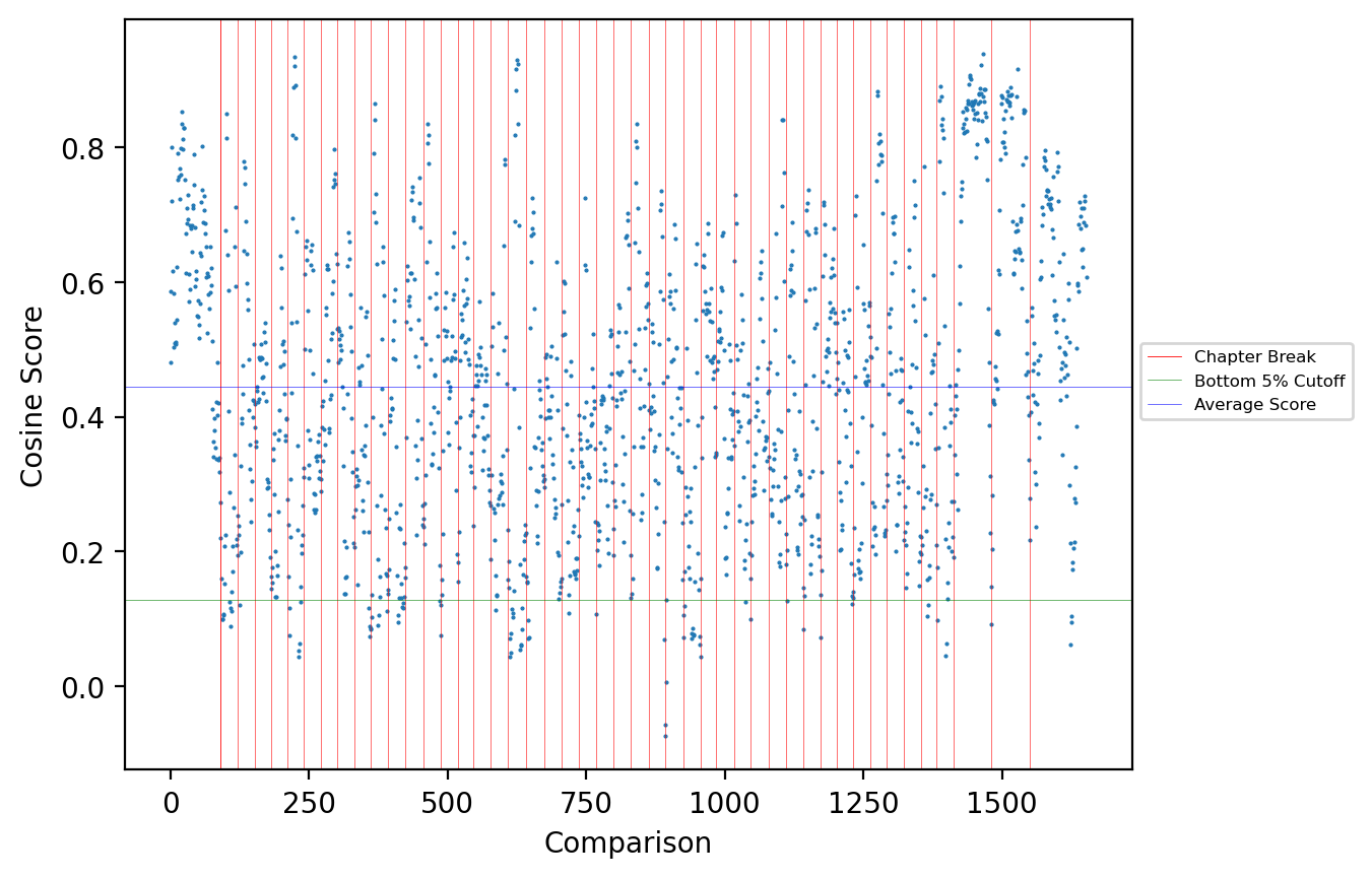
For the cleaned
Speculum experiment, the bottom
5% are represented by 82 scores, with a cosine cutoff point of approximately
0.128. The transition between the two groups of ten occurs at a chapter
break in 12% (10) of these low scores, identifying a change of topic and
explaining the low score. This value rises to 49% if we include scores where
the chapter break occurs not at the [ — ] transition but at documents that
are near it, ranging from d7 to d14. Reference to the text of the
Speculum (reading the Latin) identifies major
topic changes or unrelated content in 51% of the lowest scores. Figure 7
visualizes these results. Each dot represents the cosine comparison score
between two concatenated documents of 10 X 20, presented in order
sequentially from left to right. The vertical red lines represent chapter
divisions, and the horizontal green line represents the lowest-5% cutoff.
Upon reference to the Latin text, it becomes clear that the high scores do
indeed represent text samples that are related in content. For example, the
cluster of high scores in the upper right corner represent chapters that
record prayers directed to and describing events in the life of the Blessed
Virgin Mary. The sequence of low scores at the far right reflects the
transition of the text into a summary conclusion that leaps from topic to
topic.
Having established that the concatenation experiment successfully identified
similar and dis-similar text in addition to being sensitive to chapter
changes, we ran the same experiment on the Voynich, with intriguing results.
Overall, the similarity average was 0.483 while the average similarity over
page breaks was found to be 0.421. The average section break score (for
example at the Zodiac → Biological transition) was 0.323; this
lower-than-average score suggests that those sections could indeed be
concerned with different subjects, as suggested by the differing
illustrative content, and that the semantic space could be identifying topic
changes between sections.
In addition to section breaks, we also examined the scores at scribal
transitions. These average scores were even lower, only 0.232. Most scribal
transitions represent language (A/B) or section breaks, which explains this
result. As described above, Scribe 1 writes entirely in Language A while
Scribes 2, 3, 4, and 5 use Language B. Upon closer inspection of the scores
at scribal breaks, we observed that this method is particularly sensitive
towards scribal changes involving Scribe 1, that is, at transitions from
Language A to Language B. We had anticipated that the analysis might reveal
this distinction, although the magnitude of the distinction was surprising.
The average similarity score at A→B transitions (that is, transitions from
Scribe 1 to any other scribe and vice versa) is only 0.206, while B→B
scribal changes had a higher average score of 0.332, a substantial
difference (there are no A→A scribal transitions because Scribe 1 is the
sole user of Language A). This suggests that there is indeed a substantive
and significant difference between Language A and Language B.
Conducting the same bottom-5% analysis for the Voynich (with a cosine
similarity score cutoff point of about 0.205), we found that most of the
lowest scores can indeed be explained by reference to the manuscript itself.
Of these approximately-sixty lowest scores, 20% (12) were A→B transitions,
and 6% were section transitions. The overwhelming majority of the remaining
scores (77% or 46) were Herbal → Herbal page comparisons, virtually all of
which were near or on a page break.
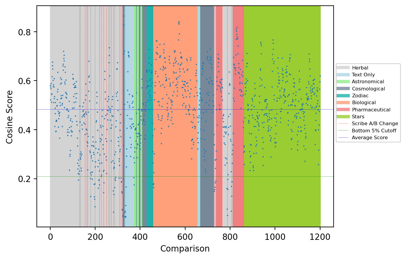
As with the
Speculum, a visualization of the
Voynich results is provided in Figure 8, with color indicating the different
sections and red vertical lines indicating A <-> B transitions. The
horizontal green line represents the lowest-5% cutoff. Upon closer
inspection, the numerous A→B scribal changes in the Herbal section (the
tight cluster of red lines) are reflected in the data, as the scores visibly
decrease and cluster in the bottom half of the gray section. Also of
interest are the higher scores in the Biological (orange), Pharmaceutical
(salmon), Zodiac (dark green), and Stars (green) sections — very few of
which are below the 5% line — indicating that these sections may concern
coherent and distinct topics.
5. Discussion
The coherence experiment was largely in line with our expectations. Our results
demonstrate that the average cosine values of correctly-ordered selections of
text are much higher than the values for the shuffled text, with a difference
that is statistically significant. This reflects the discourse coherence in the
baseline, known texts, but also suggests by extension that the Voynich
Manuscript (the dark orange and light orange columns in Figures 4-6) does indeed
demonstrate coherence across the illustrative sections in a way that is similar
to the other known texts; in other words, the proximity of words is indeed
significant. This result speaks to the overarching question of whether the
manuscript presents a semantically-interpretable text or is random nonsense. The
preponderance of evidence suggests that the manuscript may contain
semantically-interpretable text.
There are a few outliers in the results, however. For example, the results for
Dante’s Inferno, although statistically significant, are less dramatic than the
other texts present. One possible explanation for this observation may be found
in the writing style, as Dante’s Inferno is a poem with specific word and phrase
choices that may impact the results in unexpected ways. The two English
examples, Animal Farm and the Aberdeen Bestiary, also seem to have fairly different values while
the Aberdeen Bestiary scores quite high in the
ordered coherence score. Again, the explanation likely has more to do with the
style of the writing in the texts, Animal Farm
being a novel while the Aberdeen Bestiary is a
catalogue of animals and fantastical creatures; the two texts have very
different subject matter and style of delivery. The deeper investigations that
might further explain these particular results are outside the scope of this
study.
Another finding that requires explanation is that the faux-Voynich generated text
showed a very similar pattern to the Voynich Manuscript results in that they
have the same relative
“shape,” although the magnitude of the
generated Voynich scores was larger (see Figure 6 above). It is also interesting
to note the difference in hapax values between the two as well as the difference
in stop words removed; however, this will be a function of how the text is
generated. The generation of artificial text, roughly, looks at text nearby and
potentially modifies some of the words to include as generated text as it
proceeds; there is a stochastic element to this. As the artificial Voynich text
follows the
“self-citation” hypothesis put forward by
[
Timm and Schinner 2023], this might have been viewed as evidence
in favour of concluding that the manuscript has no semantic content; however,
this is offset somewhat by our findings regarding transitions from Language A to
Language B (see Figure 8 above). Their explanation of the self-citation
hypothesis states that the difference between Language A and B is a natural side
effect of the self-citation/modification of the text by the scribe over time.
The startling difference between A/B in our experiments, however, show this
change to be very abrupt and occurs mostly in the same section (Herbal) which
would seem an odd place for this to occur.
[12] Our experiments showed the opposite in the sensitivity to
the transitions between A and B, suggesting there
is a real
difference between them. It is also worthwhile to note the discourse
segmentation scores suggest that some sections contain a higher sense of
internal coherence than others (which makes sense, given the illustrative
content) — if text were truly artificially generated using a method similar to
what [
Timm and Schinner 2020] proposed, this would seem to be an odd
behaviour as we would expect a more consistent sense of coherence going through
the text, not what we are witnessing with the Voynich. The statistical skewness
and kurtosis values of the Voynich raw cosine scores (with TF-IDF 40 values for
example) are very different than those calculated for the artificially generated
values too suggesting a different underlying pattern and distribution (0.48/0.44
vs 0.06/-0.63). The Voynich, for example, has circular and radial text on some
of its pages and the algorithm used to create artificial Voynich does not try to
simulate things such as this. However, a scribe using such a system would have
freedom as to how and when to
“make changes.”The discourse segmentation results were enlightening (see Figure 7 above). For
the
Speculum, we see there is generally a drop in
scores at the Chapter breaks, which is to be expected and falls in line with the
results of [
Foltz, Kintsch, and Landauer 1998] in their experiments they recorded. We
could also explain the cluster of high scores in the upper right of Figure 7 as
well as the sequence of increasingly-low scores at the end of the text by
referring back to the text itself. The overall behavior would seem to confirm
LSA is working as expected. In the Voynich Manuscript we see that the Herbal
section appears to have some minor coherence at the beginning, coherence that
deteriorates quickly once the text transitions from and between language A and
B. This LSA sensitivity to the difference between A and B was startling. This
observation has implications for the LSA semantic space, as identical words that
may be used in a substantially different way in A and B pages could suppress the
scores in comparisons that include documents in both Language A and B; this may
be a topic for future experiments.
Several potentially important conclusions can be drawn from the Voynich results
expressed in Figure 8 (above):
- Herbal section: Beginning with the first A→B transition, the scores show a
marked decrease, suggesting that the A→B transition is significant.
- Cosmological, Astronomical, and Astrological sections: The documents in
this section (written entirely in Language B) behave similarly to the
Language A section of the Herbal portion of the manuscript, that is, they
record slightly lower than average scores at page transitions. As each
diagram in these sections are unique (and uninterpreted as of yet), we can
conclude from this analysis that each page is likely a different topic. In
the astrological section, this contention is supported by the images, which
focus on a different zodiac sign on each page.
- Biological, Pharmaceutical, and Stars sections: The results in these
sections seem to clearly indicate a marked textual cohesion in each of these
three sections, as they show mostly above-average scores with very few
scores in the lowest 5%. This reflects the internal cohesion suggested by
their illustrative content (for the Biological and Pharmaceutical sections)
and common format (for the Stars section).
6. Conclusions
The application of Latent Semantic Analysis to the text of the Voynich Manuscript
has proven to be a productive and novel method of analyzing the contents of the
manuscript. We have demonstrated the effectiveness of the method by applying it
to several known texts and manuscripts, established the general quality of
coherence and flow across the Voynich Manuscript, and uncovered previously
unseen and surprising features of the Voynich text.
In particular, we have demonstrated that the Voynich Manuscript seems to follow a
coherence pattern similar to known texts. That is, text samples that are closer
together, in general, have a higher
“similarity
score” than text samples that are farther apart. The difference
between the known texts and Voynich text is that with known text we can refer
back to the text to explain the results — high similarity scores do indeed
generally reflect topical similarity. With the Voynich Manuscript we cannot
check our results, but, even so, these results allow us to speculate that there
may indeed be semantic content in the manuscript. The discourse segmentation
analysis also revealed interesting patterns, showing how several sections of the
manuscript seem to have topical coherence reflected in their internal similarity
scores while others, such as the Cosmological and Astronomical sections, seem to
change sub-topics with each page turn. Languages A and B, on the other hand, are
shown to display a surprising degree of
dissimilarity, a result
that directly contrasts with some research in this area but that supports other
results [
Lindemann and Bowern 2021].
The present collaboration between a computer scientist (Layfield) and a medieval
codicologist (Davis) demonstrates the importance of interdisciplinary
methodologies where the Voynich Manuscript is concerned. The manuscript is such
a complex object that no one person could hope to master all of the fields
necessary to undertake a thorough investigation of its contents, illustrations,
structure, and history. Neither of the present authors could have reached these
results without the other. Scientific and humanistic collaboration is crucial.
It is only by reaching across the disciplinary divides that we will be able to
make progress in understanding the mysteries of the Voynich Manuscript.
The present study has investigated the coherence and flow of the Voynich
Manuscript from a big-picture perspective; in forthcoming work (currently under
review), the authors will present more granular results that consider how LSA
can shed light on the original codicological structure of the manuscript. It is
our hope that these results will assist others in their work on the Voynich
Manuscript, moving us all closer to a deeper understanding of the World’s Most
Mysterious Manuscript.
Appendix 1: History and Methodology of LSA
Methodology
In order to generate our semantic space, we first need a set of \(m\) terms and \(n\)
documents. The list of
terms should be all the unique terms from the collection of text overall.
The documents should be the set of documents (these can range from sentences
and paragraphs to an entire large piece of text) from which we wish to
create our semantic space. From this dataset we generate a \(m\) by \(n\) (term by
document) matrix \(A\). Each \(A_{ij}\) value in this matrix indicates the number of times
term \(i\) occurs in
document \(j\), the
so-called Term Frequency (TF).
The next step is to compute the Singular Value Decomposition (SVD) of the
Matrix \(A\). This is a form
of factor analysis and factors our matrix \(A\) into three matrices: $$A = TSD^{T}$$
These matrices have the following shape:
For a full mathematical description of the factors, the reader is referred to
the original paper [
Deerwester et al. 1990]. The \(T\) and \(D^T\) matrices will be almost entirely
nonzero, and the \(S\)
matrix is actually a diagonal matrix of the singular values from the
computation in descending order.
Roughly speaking, the \(D^T\)
matrix refers to the documents from which we have built this space. Each
column corresponds to the document in the column space of \(A\) (which, most importantly,
is
non sparse). The next step in this process is the
dimensionality reduction phase. This involves picking a value, \(k\), and reducing
the
dimensionality of our \(T\),
\(S\) and \(D^T\) matrices such that they
are \(m\) X \(k\), \(k\) X \(k\), and \(k\) X \(m\)
— that is we keep the first \(k\) columns in \(T\), the first \(k\) values in the
diagonal matrix \(S\) and the first \(k\) rows in \(D^T\). This results in an approximation
of
\(A\). More importantly,
we reduce the dimensionality in order to filter out some of the noise in the
space and focus on the key relationships found within. The selection of this
value is somewhat subjective. In the work by [
Foltz, Kintsch, and Landauer 1998], they use a value
of 300 for \(k\) as their
original \(A\) matrix is of
a moderate size. There are some suggested methodologies for computing an
appropriate value of \(k\)
(such as choosing a \(k\)
such that the ratio of the sum of the squares of the first \(k\) singular values divided
by
the sum of the entire set of squared singular values is about 0.8), but we
have found that for smaller datasets they tend to work quite poorly. As the
term-by-document matrices we will be dealing with (such as the text from the
VM) we have used a value of 75 for \(k\). Note the matrices we will be using are much
smaller
than the ones used in the original experiment in [
Foltz, Kintsch, and Landauer 1998]
so a smaller dimensionality is justified. We give a justification of this
value next.
The dimensional reduction step in LSA involves a selection of the number of
dimensions to use from the SVD decomposition. This is a tricky choice, and
much of the literature (especially in the context of Information Retrieval
(IR)) suggests you pick a \(k\) that gives you the best results (for a typical
train/test split for an IR problem this is straightforward). As we don’t
know the contents of the Voynich, this is clearly impossible, so we use
three heuristics to approximate what might be a good value for \(k\) by calculating
what might
be a good lower, mid, and upper bound selection of values. This is actually
done for all the dataset’s semantic spaces. Note, these heuristics are
designed for a semantic space generated from a
single text
which may not be typical in general. Given the results from [
Foltz, Kintsch, and Landauer 1998], we know that sequential document comparisons
should have a larger value than the shuffled variant as per our first
experiment; so we first calculate a coherence score which is the average
similarity of adjacent documents in the \(D^T\) matrix. Next, we shuffle the order
of
the documents in \(D^T\) and
make the same calculation (random) and do this 10 times taking the average.
This is like our coherence experiment except we are using this to help
calibrate \(k\). We then use
three different techniques to approximate \(k\).
1. Noise separation: Compare the baseline coherence for a dimension with the
random baseline. Select the \(k\) with the largest difference (indicates strong semantic
pattern). This would act as the lower bound for \(k\) as typically the difference
is largest the
smaller the dimension (assuming the text has any coherence). If the
dimension selected is quite low this runs the risk of over-simplification
and causing the model to lose essential topic/latent information.
2. Elbow detection: Find point of diminishing returns in the coherence
scores. This is often indicated by the “elbow” of the
coherence scores over the range of \(k\) explored. The similarity scores at this point
begin to
taper off. This is typically the default value of \(k\) as it should be larger than
the Noise
separation value and smaller than the Slope stabilization value.
3. Slope stabilization: Identify when the coherence values begin to flatten
out. As the dimension increases usually the scores decrease. When the scores
flatten out additional dimensions contribute very little. This is typically
the upper bound for a reasonable \(k\).
We ran these heuristics over a \(k\) range of [25, 200]. We did this for all datasets
used,
TF, TF-IDF and Log-Entropy weighting methods as well as document sizes of
20, 30 and 40. The range of values for the noise separation methods was [25,
30], for elbow detection it was [65, 90] and for the slope stabilization
method it was [115, 160]. A reasonable range for \(k\) would seem to be 65-90 and
as the average
value for the elbow method, overall, was 75 so that was selected as the
dimension to use for all the semantic spaces (anything in the range 65-90
should work reasonably well).
To compare two documents in the \(D^T\) matrix we need to generate two vectors to
perform the
cosine operation on. If we wanted to compare document \(i\) and \(j\) (corresponding
to columns \(i\) and \(j\)) we would generate their vectors as
follows: $$\vec{v_{i}} =
S_{k}D^{T}_{ki}$$
$$\vec{v_{j}} =
S_{k}D^{T}_{kj}$$
Each vector is comprised of the product of the \(S\) matrix (singular values) and
the
appropriate column in the \(D^T\) matrix. The subscript \(k\) indicates we are using
the first \(k\) dimensions.
Then apply the cosine operator as follows: $$\cos(\vec{v_{i}}, \vec{v_{j}}) = \frac{\vec{v_{i}}
\cdot
\vec{v_{j}}}{\| \vec{v_{i}} \| \| \vec{v_{j}} \|}$$ We can
also compare documents that do not already exist as columns in the document
semantic space. This is achieved via a process known as
“folding-in” a document which essentially transforms
it into the same vector space as the documents that already exist in
\(D^T\). So given a new
document, \(d\), that we
want to use for comparison purposes, we put it into the same format as a
column in the original A matrix; that is, each dimension of \(d\) indicates how many
times a
particular term occurs in the document. We then fold it into the \(D^T\) matrix (essentially
as an
extra column) as follows: $$\vec{d^{1}}
= \vec{d}T_kS_k^{-1}$$ At this point, the new document vector
\(\vec{d^{1}}\) can be
treated just as any other document vector in \(D^T\) for comparison purposes.
Building the Models for the Coherence Experiment
One question that has yet to be answered is: What do we consider a
“document” in the context of generating our initial
term-by-document matrices? For the original coherence experiments in [
Foltz, Kintsch, and Landauer 1998], they used a document size of one sentence and,
in the discourse segmentation part of their experiments, they used
collections of 10 paragraphs as a document unit. With the VM we have no real
concept of
“sentence” as there appears to be no
punctuation in the writing. Bearing this in mind (and wanting to treat all
documents equally) we opted to experiment with document sizes of 20, 30 and
40 terms respectively. These are simply constructed by taking term sets of
20, 30 and 40 terms from the processed texts and treating those as the
document partitions for creating the initial term-by-document matrix
\(A\).
We experiment by applying additional NLP techniques to the \(A\) matrix to try and
lessen
the effect of more common terms in the comparisons. There is potentially a
problem in only utilizing TF values in the \(A\) matrix in that very common terms
will have
more influence in comparison operations then perhaps they should, purely due
to their common appearance over the text. Removal of stop words partially
resolves this issue, but there will still be a disproportionately high
presence of some terms over others. In addition to creating the \(A\) matrix as described,
which
uses straight TF values, two weighting schemes are also employed to modify
the values contained in \(A\). The two schemes applied are Term Frequency-Inverse
Document Frequency (TF-IDF) and Log-Entropy (LE).
Log-Entropy is defined in Equation 5 (in the context of matrix \(A\)). \(f_{ij}\)
represents the TF of term \(i\) in document \(j\) and \(p_{ij} = \frac{f_{ij}}{\sum_{j}f_{ij}}\)
which
equates to the fraction of occurrences term \(i\) has in document \(j\) over all occurrences
of term \(i\) and \(n\) is the number of documents (columns) in
\(A\). Log-Entropy was
the matrix weighting mechanism used in the experiments by [
Foltz, Kintsch, and Landauer 1998]. The first logarithm decreases the effect of the
differences in term frequency (to help smooth them out) whilst the entropy
calculation will tend to give less weight to frequently occurring terms;
additionally, it takes the distribution of the terms over the document set
into account. $$A_{ij} = \log(1 +
f_{ij}) \left[ 1 + \left(\sum_{j}
\frac{p_{ij}\log(p_{ij})}{\log(n)}\right) \right]$$ TF-IDF is
defined in Equation 6. The value \(df_i\) represents the document frequency of term
\(i\); that is, the number of
unique documents that term \(i\) occurs in. The logarithm value is the inverse document
frequency, and it is high if the term is rare, thus emphasizing the value of
rare terms and de-emphasizing the values of common terms. $$A_{ij} = f_{ij} \log{\left(
\frac{n}{
df_{i} } \right) }$$ It is worth noting that each semantic
space is trained on its own document and comparisons/experimentation is done
within that semantic space. This can be viewed as a
circular
relationship or, perhaps better stated, self-contained distributional
modelling (in the sense the training data is what we are working on) and can
potentially viewed as problematic. Our experiments are
not
testing
generalization (an issue with over-fitting); instead,
we are testing internal structure. The goal of our work is to characterise
internal coherence and discourse structure rather than consider predictive
performance or any sense of generalization; that is, do the different
semantic spaces behave in a similar fashion?
There is also some precedence of the usage of a generated semantic space and
experimentation on the same space with the data it was trained on. [
Dos Santos and Favero 2015] built a LSA semantic space from a set of
student answers to exam questions. They evaluated the performance of this on
the same dataset (comparing human assigned scores to computer generated
scores) and reported an 85% agreement with human scoring. [
Altszyler et al. 2017] applied LSA using a semantic space made up of
dream reports analysing usage patterns of words between dreams and waking
life (the analysis making use of the same semantic space data). They also
compared the results with Word2Vec deducing that with smaller corpus sizes
Word2Vec becomes less effective compared to LSA. In addition, the paper [
Foltz, Kintsch, and Landauer 1998], from which we are taking our methodology, both
for coherence and discourse segmentation, literally uses a semantic space
trained on a dataset and then performs discourse segmentation on this space
using the same dataset (no external data was used for training) which is
exactly what we are doing.
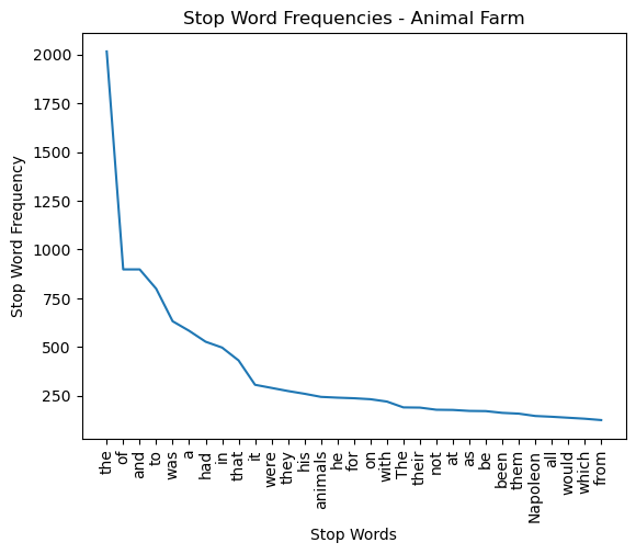
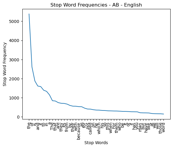
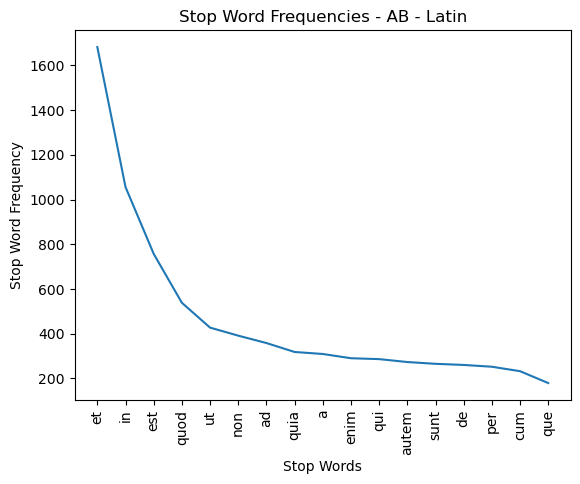
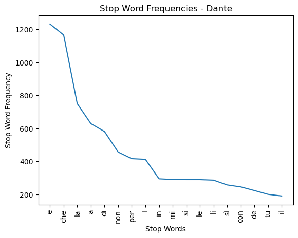
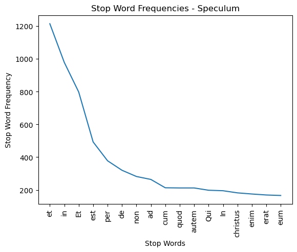
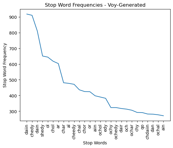
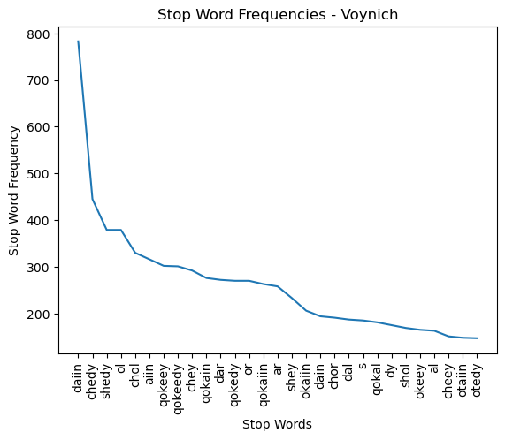
Generating Stop-Word Lists
In order to generate a stop word list, terms are sorted by their Term
Frequency (TF) count in descending order. Using a window of size \(w\), we calculate
the average
difference in TF between the first \(w\) terms in our list. We move this window by
1 word and
calculate this difference again. This process is repeated until this
difference falls below a threshold value of \(v\). If \(x\) steps were required to
reach this threshold value, the
first (\(w + x – 1\)) words
in our list are selected as our stop words. In other words, we look at the
average decrease in the TF in a moving window until the rate of change falls
below some value \(v\). We
utilize a window of size 6 and a threshold of 3 to generate reasonable stop
word lists for English, Medieval Italian and Latin (essentially the top most
frequent words given the cutoff threshold defined above). The VM stop word
list is calculated using the same process and parameters. The stop word
lists and their term frequencies are shown in Figures 10 through 16:
Notes
[1] F. 116v is not part of the primary text
and will not be considered here.
[2] The Appendix contains justification for the
selected dimensional reduction as well as potential issues around how the
semantic spaces themselves are constructed.
[3] Such as Term Frequency-Inverse Document
Frequency (TF-IDF) or Log-Entropy. These are defined in Appendix 1.
[4] Again, TF-IDF and Log-Entropy are defined in Appendix
1.
[5] All the datasets used are described in Section 3.1
[6] The partition is split up into documents that, on
average, are as close to 20 or 40 as possible as it’s unlikely the text is
exactly divisible by these values - text sections that are, in their
entirety, less than half the target size, 20/40, are discarded.
[9] The text generated using Timm and Schinner’s process used the
default parameters except for “lines_to_create” where the value 3,500 was substituted (to
generate more text) and the parameter “method.canFollow” which was set to the value
“statistic” as this bases the generated text on
the statistics for the VM.
[11] The original [Foltz, Kintsch, and Landauer 1998] paper used a cutoff point of 2 standard deviations - as our results do not follow
a normal distribution, this would have made little sense, so we chose a cutoff point
of 5%.
[12]
[Timm and Schinner 2020] suggest an alternative ordering of the
manuscript to account for the change in text over time. This would place
Herbal A and Herbal B apart from each other, with several sections in
between.
Works Cited
Altszyler et al. 2017 Altszyler, E., Sigman,
M., Ribeiro, S. and Slezak, D.F. (2017)
“The interpretation
of dream meaning: Resolving ambiguity using latent semantic analysis in
small corpus of text”,
Consciousness and
Cognition, 56, pp. 178–187. Available at:
https://doi.org/10.1016/j.concog.2017.09.004
Davis 2020 Davis, L.F. (2020)
“How many glyphs and how many scribes? Digital paleography and the Voynich
manuscript”,
Manuscript Studies: A Journal of
the Schoenberg Institute for Manuscript Studies, pp. 164–180.
Available at:
https://doi.org/10.1353/mns.2020.0011
Deerwester et al. 1990 Deerwester, S.,
Dumais, S., Furnas, G., Landauer, T. and Harshman, R. (1990)
“Indexing by latent semantic analysis”,
Journal of the American Society for Information
Science, pp. 391–407. Available at:
https://doi.org/10.1002/(SICI)1097-4571(199009)41:6%3C391::AID-ASI1%3E3.0.CO;2-9
Dos Santos and Favero 2015 Dos Santos, J.C.A.
and Favero, E.L. (2015)
“Practical use of a latent semantic
analysis (LSA) model for automatic evaluation of written answers”,
Journal of the Brazilian Computer Society,
21(21). Available at:
https://doi.org/10.1186/s13173-015-0039-7
Foltz, Kintsch, and Landauer 1998 Foltz, P.,
Kintsch, W. and Landauer, T. (1998)
“The measurement of
textual coherence with latent semantic analysis”,
Discourse Processes, pp. 285–307.
https://doi.org/10.1080/01638539809545029
Landauer and Dumais 1997 Landauer, T.
and Dumais, S. (1997)
“A solution to Plato's problem: The
latent semantic analysis theory of acquisition, induction, and
representation of knowledge”,
Psychological
Review, pp. 211–240. Available at:
https://psycnet.apa.org/doi/10.1037/0033-295X.104.2.211
Lindemann and Bowern 2021 Lindemann, L.
and Bowern, C. (2021)
“Character entropy in modern and
historical texts: Comparison metrics for an undeciphered manuscript”.
Available at:
arXiv:2010.14697v2.
Manly 1921 Manly, J. (1921) “The most mysterious manuscript in the world”, Harper's Magazine, pp. 186–197.
Pelling 2006 Pelling, N. (2006) The curse of the Voynich. Surbiton: Compelling
Press.
Reddy and Knight 2011 Reddy, S. and Knight,
K. (2011)
“What we know about the Voynich
manuscript”, in
Proceedings of the 5th ACL-HLT
Workshop on Language Technology for Cultural Heritage, Social Sciences, and
Humanities, June 2011, pp. 78–86. Available at:
http://dl.acm.org/citation.cfm?id=2107647.
Sterneck, Polish, and Bowern 2021 Sterneck, R.,
Polish, A. and Bowern, C. (2021)
“Topic modeling in the
Voynich manuscript”. Available at:
arXiv:2107.02858.
Vaswani et al. 2017 Vaswani, A., Shazeer, N.,
Parmar, N., Uszkoreit, J., Jones, L., Gomez, A., Kaiser, L. and Polosukhin, I.
(2017) “Attention is all you need”, in 31st Conference on Neural Information Processing Systems (NIPS
2017), Long Beach, CA, USA.
Zandbergen 2004–2025 Zandbergen, R. (2004–2025)
The Voynich manuscript.
Available at:
https://www.voynich.nu/ (Accessed: 12 February 2025).
Zandbergen 2020. Zandbergen, R. (2020) “IVTFF intermediate Voynich MS
transliteration file format: File format 2.0”.